MonoTools.fit is the key class needed to implement the fitting of planets with unconstrained periods.
It works by first building a fit objects, and telling it the lightcurve, stellar parameters, rvs, etc to use, as well as the planets to model.
It then enables a range of fitting, plotting, and outputs.
[1]:
from MonoTools import fit
from MonoTools import lightcurve as lc
import numpy as np
import matplotlib.pyplot as plt
%matplotlib inline
%load_ext autoreload
%autoreload 2
Matplotlib created a temporary config/cache directory at /var/folders/p0/tmr0j01x4jb3qrbc5b0gnxcw0000gn/T/matplotlib-tyrjjtpm because the default path (/Users/hosborn/.matplotlib) is not a writable directory; it is highly recommended to set the MPLCONFIGDIR environment variable to a writable directory, in particular to speed up the import of Matplotlib and to better support multiprocessing.
Using MonoTools.fit for a simulated “Duotransit”
Using simulated data
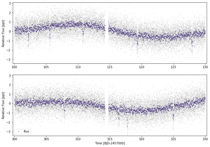
Let’s just put together some fake data where we know the answer and see what we get out! Here’s 2 pseuod-sectors of TESS data, and planets at 8d & 35d.
[2]:
x = np.concatenate((np.arange(100,114.25,2/1440), np.arange(114.75,130,2/1440),
                    np.arange(300,314.25,2/1440), np.arange(314.75,330,2/1440)))

#Adding some randomised sinusoids to mimic stellar variability:
y_sv=abs(np.random.normal(0.0002,0.0005))*np.sin((x+np.random.random()*2*np.pi)/(np.random.normal(8,1)))+abs(np.random.normal(0.0001,0.0005))*np.sin((x+np.random.random()*2*np.pi)/(np.random.normal(3,0.8)))

#Now adding noise to the lightcurve
noise=0.0008
y = np.random.normal(1.0,noise,len(x))+y_sv
yerr = noise*1.1+np.zeros_like(y)

it0s=np.array([np.random.random()*8.56781,105.57])

#Depth here is a little over double the per-point scatter
idepths=np.array([0.0007,0.0018])
import exoplanet as xo
true_orbit = xo.orbits.KeplerianOrbit(period=np.array([8.56781,35.36789]),
                                      t0=it0s, b=np.random.random(2),
                                      omega=np.random.random(2)*2*np.pi, ecc=np.random.random(2)*0.05)
true_model = np.sum(xo.LimbDarkLightCurve([0.3, 0.2]).get_light_curve(orbit=true_orbit, t=x, r=np.sqrt(idepths)).eval(),axis=1)
y += true_model

lc1=lc.lc();lc1.load_lc(time=x[:21240], fluxes=y[:21240], flux_errs=yerr[:21240],
                        flx_system='norm1',jd_base=2457000,mission='tess',sect='98',src='test')
lc2=lc.lc();lc2.load_lc(time=x[21240:], fluxes=y[21240:], flux_errs=yerr[21240:],
                        flx_system='norm1',jd_base=2457000,mission='tess',sect='99',src='test')
ilc=lc.multilc(123456789,'tess',do_search=False,load=False)
ilc.stack([lc1,lc2])

#plotting the data:
ilc.plot(plot_rows=2)
Initialising a fit object
First thing to do is to intialise the fit object. This requires id and mission arguments.
These help point MonoTools where to save/access data. MonoTools will access the $MONOTOOLSDATA system environment variable for custom data locations, but will default to store data in MonoTools/data where the module is stored. For each id/mission pair, MonoTools will create a fresh directory to store all data with the form [KIC/TIC/EPIC][zero-padded 11-digit ID], i.e.MonoTools/data/TIC00100990000`.
[3]:
mod = fit.monoModel(123456789,'tess',lc=ilc)
Adding stellar parameters
We need to makesure our star is defined. A good stellar density can especially help constrain the periods of planets on unconstrained orbits.
By default, these are taken from the data within a MonoTools.lightcurve.multilc object (i.e. from the TIC), but if we do not have that, as here, we need to initialise the stellar parameters directly.
Using init_starpars we must include a Rstar and Teff input, and then one or two of logg, rhostar or Mstar (if not, the other one or two of these parameters are calculated from the known params):
[4]:
mod.init_starpars(Rstar=[0.98,0.05,0.05],
                  rhostar=[1.02,0.1,0.1],
                  Teff=[5660,120,120])
Adding planets to the model:
To initialise the planets to fit, we have a couple of options. Either we run one of the three planet types directly, namely add_multi (multi-transiting planet with a contrained period), add_duo (duo-transiting planet with two transits), and add_mono (single-transiting candidate). There is also add_rvplanet for an RV-only Keplerian signal.
In this case, we add the duo by specifying the transit times of each transit, the depth, and a duration in a dictionary, as well as our name for the planet like so:
[5]:
mod.add_duo({'tcen':105.57,'tcen_2':317.78,'tdur':0.275,'depth':idepths[1]},'c')
Or we can use the add_planet function which wraps all four of these options (so long as we specify in the function which type we want).
For multi-transiting planets, we also need to specify a period (obviously) and a period error (not so obviously) which helps loosely constrain the fitting priors.
[6]:
mod.add_planet('multi',{'tcen':it0s[0],'period':8.567,'period_err':0.005,'tdur':0.12,'depth':idepths[0]},'b')
Accessing planet data
The initial planetary data is stored as dictionaries in mod.planets:
[ ]:
mod.planets
Performing an initial model fit
Now we have the planets we want to model, let’s initialise the model itself and obtain a best-fit we can inspect.
We do that using init_model().
These are the key arguments to be aware of: * use_GP: Whether to fit a GP in parrallel to the transit fit. If yes (and train_GP=True) we train a SHO celerite2 kernel on out-of-transit data and then co-fit with the data. If not, we perform spline fitting to out-of-transit data and flatten the lightcurve. * bin_oot: Whether to bin the out-of-transit points. This reduces compute time. Default = True * cut_distance: How far from each transit (in durations) to either “cut” or
“bin”. * interpolate_v_prior: Whether to fit only for the transit shape parameters and use interpolation to map this to orbital period. Default: True * ecc_prior: Which eccentricity prior to use for the interpolation (‘uniform’, ‘kipping’, ‘vaneylen’, or the default ‘auto’, which chooses between kipping & vaneylen based on multiplicity).
[7]:
mod.init_model()
#This can be reasonably slow, as we have to:
#   1) train the GP and then 2) progressively minimize more and more parameters in the combined model
initialising and training the GP
4.1887902047863905 96.40483785469252 0.6283185307179586 {'alpha': 6.570746817359475, 'beta': 8.763441085702263} 1.157539843441598
0.36916761081013877 0.36916761081013877 0.7525577544224005
optimizing logp for variables: [phot_mean, phot_w0, phot_power, logs2]
message: Optimization terminated successfully.
logp: -52.09461968896364 -> -0.77344119054942
Multiprocess sampling (2 chains in 4 jobs)
NUTS: [phot_power, phot_w0, logs2, phot_mean]
Sampling 2 chains for 594 tune and 900 draw iterations (1_188 + 1_800 draws total) took 22 seconds.
ts
ts
optimizing logp for variables: [b_b, logror_b, tdur_c, b_c, logror_c]
message: Desired error not necessarily achieved due to precision loss.
logp: -9256.560591192092 -> -8886.45446053474
optimizing logp for variables: [per_b, logror_b, t0_2_c, logror_c]
message: Desired error not necessarily achieved due to precision loss.
logp: -8886.45446053474 -> -8840.288083568093
optimizing logp for variables: [omega_b, ecc_b, b_b, logror_b, t0_b, tdur_c, b_c, logror_c, t0_c, logrho_S]
message: Desired error not necessarily achieved due to precision loss.
logp: -8840.288083568095 -> -8806.525492397373
optimizing logp for variables: [phot_mean, phot_w0, phot_power, logs2]
message: Desired error not necessarily achieved due to precision loss.
logp: -8806.525492397372 -> -8795.922317173929
optimizing logp for variables: [per_b, b_b, logror_b, tdur_c, b_c, logror_c]
message: Desired error not necessarily achieved due to precision loss.
logp: -8795.922317173929 -> -8795.222765315853
optimizing logp for variables: [u_star_tess, logrho_S, Rs, logs2, phot_mean, phot_w0, phot_power, omega_b, ecc_b, b_b, logror_b, t0_b, tdur_c, b_c, logror_c, t0_c]
message: Desired error not necessarily achieved due to precision loss.
logp: -8795.222765315853 -> -8794.684330132783
optimizing logp for variables: [phot_mean, phot_power, phot_w0, logs2, u_star_tess, b_b, omega_b, ecc_b_frac, ecc_b_sigma_rayleigh, ecc_b_sigma_gauss, ecc_b, logror_b, per_b, t0_b, tdur_c, b_c, logror_c, t0_2_c, t0_c, Rs, logrho_S]
message: Desired error not necessarily achieved due to precision loss.
logp: -8794.684330132783 -> -8792.273722947479
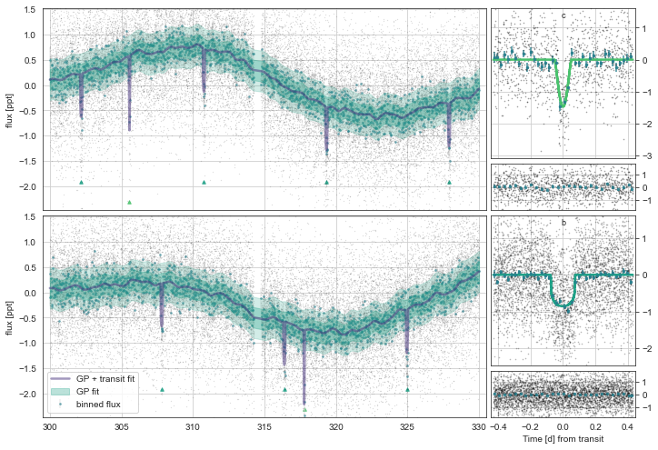
Plotting the initial model
We can now plot the initial minimized model. This plots both the lightcurves and a zoom at the phase-folded transits
[8]:
mod.Plot(n_samp=1)
initialising transit
Initalising Transit models for plotting with n_samp= 10
Initalising GP models for plotting with n_samp= 1
successfully interpolated GP means

Sampling with PyMC
This uses the exoplanet/PyMC3 NUTS sampler under the hood, which should provide chains with far higher effective samples compared to MCMC, and the PyMC3_ext implementation allows for correlations to be trained/learned.
Some important arguments: * n_draws - number of samples to take per chain * n_burn_in - number of samples which will constitute the “burn-in” (in the default case, this is 2/3 n_draws) * overwrite - whether to start fresh or load a saved model * continue_sampling - whether to start from the MCMC trace already saved within the model * chains - number of chains to sample (defaults to 4)
[9]:
mod.SampleModel(n_draws=1333)
Multiprocess sampling (4 chains in 4 jobs)
NUTS: [phot_mean, phot_power, phot_w0, logs2, u_star_tess, b_b, omega_b, ecc_b_frac, ecc_b_sigma_rayleigh, ecc_b_sigma_gauss, ecc_b, logror_b, per_b, t0_b, tdur_c, b_c, logror_c, t0_2_c, t0_c, Rs, logrho_S]
Sampling 4 chains for 879 tune and 1_333 draw iterations (3_516 + 5_332 draws total) took 3272 seconds.
Saving sampled model parameters to file with shape: (127, 14)
[10]:
mod.Plot(n_samp=101)
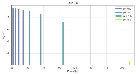
[11]:
mod.PlotPeriods()
[12]:
df=mod.MakeTable()
df
Saving sampled model parameters to file with shape: (127, 14)
[12]:
| mean | sd | hdi_3% | hdi_97% | mcse_mean | mcse_sd | ess_bulk | ess_tail | r_hat | 5% | -$1\sigma$ | median | +$1\sigma$ | 95% | |
|---|---|---|---|---|---|---|---|---|---|---|---|---|---|---|
| Rs[0] | 1.00002 | 0.05018 | 0.90178 | 1.09296 | 0.00073 | 0.00052 | 4762.06164 | 3486.56172 | 1.00048 | 0.91665 | 0.95029 | 1.00004 | 1.04953 | 1.08244 |
| per_b | 8.56762 | 0.00013 | 8.56738 | 8.56785 | 0.00000 | 0.00000 | 4117.37595 | 3287.41837 | 1.00041 | 8.56741 | 8.56750 | 8.56762 | 8.56774 | 8.56781 |
| logs2[0] | -4.61820 | 0.11593 | -4.86032 | -4.42118 | 0.00175 | 0.00124 | 4552.05885 | 3293.66915 | 1.00017 | -4.82146 | -4.73309 | -4.61235 | -4.50312 | -4.43814 |
| rho_S | 0.99957 | 0.09460 | 0.82539 | 1.17588 | 0.00181 | 0.00128 | 2706.92618 | 2759.04023 | 1.00152 | 0.84542 | 0.90274 | 0.99826 | 1.09282 | 1.15521 |
| Ms[0] | 1.00755 | 0.18183 | 0.69458 | 1.36310 | 0.00296 | 0.00209 | 3769.78214 | 3726.01701 | 1.00028 | 0.73662 | 0.82663 | 0.99425 | 1.18580 | 1.32635 |
| ... | ... | ... | ... | ... | ... | ... | ... | ... | ... | ... | ... | ... | ... | ... |
| logprob_c[7] | -1.98908 | 15.90281 | -10.37283 | 2.12143 | 0.42148 | 0.29809 | 453.08112 | 1012.71069 | 1.01755 | -11.60142 | -4.85724 | 0.87274 | 1.80287 | 2.07808 |
| ecc_c | 0.54311 | 0.06803 | 0.40762 | 0.65214 | 0.00373 | 0.00264 | 397.40728 | 804.58241 | 1.01610 | 0.41178 | 0.47088 | 0.55303 | 0.61213 | 0.63628 |
| ecc_marg_c | 0.54311 | 0.06803 | 0.40762 | 0.65214 | 0.00373 | 0.00264 | 397.40728 | 804.58241 | 1.01610 | 0.41178 | 0.47088 | 0.55303 | 0.61213 | 0.63628 |
| vel_marg_c | 1.00109 | 0.03196 | 0.96338 | 1.06398 | 0.00108 | 0.00077 | 784.04144 | 2315.61306 | 1.00950 | 0.97163 | 0.97712 | 0.98574 | 1.03774 | 1.06505 |
| per_marg_c | 35.18867 | 8.78527 | 26.63492 | 52.32191 | 0.51564 | 0.36498 | 400.99617 | 818.74112 | 1.01554 | 27.15514 | 28.12749 | 31.89983 | 44.05159 | 54.85980 |
127 rows × 14 columns
The “true” period is one of the highest-probability. And the “marginalised period” for the planet (i.e. an average of all period aliases weighted by their respective probabilities) is close to the true value!
Using MonoTools.fit on real “Duotransits”
Let’s try MonoTools out with some real data. Let’s use TOI-2076, which has two Duo-transiting planets (see Hedges et al 2021 and Osborn et al. 2022).
Here, unless we specify otherwise, the monoModel will load a TESS lightcurve (as a MonoTools.lightcurve.multilc object), as well as stellar parameters from the TIC.
[2]:
mod = fit.monoModel(27491137,'tess')
Getting all IDs
Empty TableList
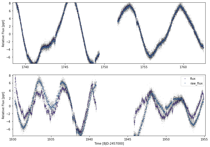
Using the lc.plot() feature.
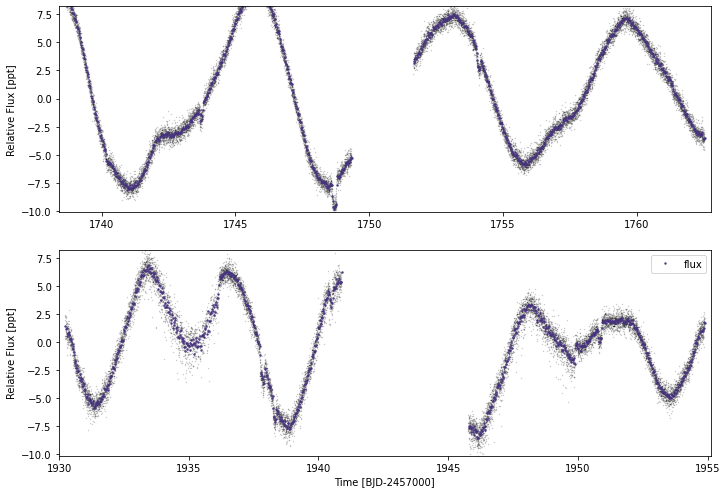
Here we can see that SPOC really fails in the PDC detrended flux for the second sector. Let’s just use the raw flux there instead
[3]:
mod.lc.plot(timeseries=['flux','raw_flux'])
[4]:
mod.lc.flux[mod.lc.cadence=='ts_120_pdc_23']=mod.lc.raw_flux[mod.lc.cadence=='ts_120_pdc_23']
#Need to re-bin
mod.lc.bin()
[5]:
mod.lc.plot()
That looks better. Although there is still some excess scatter on the second sector.
[6]:
mod.add_multi({'tcen':1743.7199,'period':10.356192390280784,'period_err':0.0025,
                   'tdur':3.25/24,'depth':1.4e-3},'b')
mod.add_planet('duo',{'tcen':1748.675688904365,'tcen_2':1937.821199104365,
                      'tdur':4.186/24,'depth':2.0e-3},'c')
mod.add_duo({'tcen':1762.6651396199247,'tcen_2':1938.2899096646295,
                 'tdur':3.046/24,'depth':1.4e-3},'d')
By default, the model bins the out-of-transit lightcurve and performs a GP fit on all of the data. But we can manipulate how MonoTools performs the fit.
Here let’s turn off the GP and only use a zoomed-in view of a detrended/flattened lightcurve for each of the transits using bin_oot = False and cut_distance=3.5. This should also be quicker. We specify a “knot distance” knot_dist of 0.6 for the spline as this is a very wiggly lightcurve!
[8]:
mod.init_model(use_GP=False,
               bin_oot=False,
               cut_distance=3.5,
               knot_dist=0.6)
yerr __str__ = [0.63242328 0.63232464 0.63244091 ... 0.6402334 0.64008134 0.64026565]
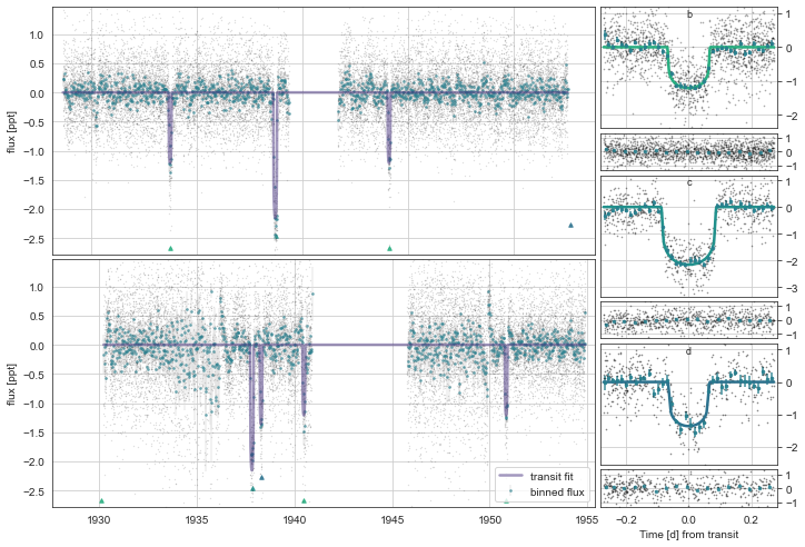
Let’s plot the initial model:
[9]:
mod.Plot(plot_flat=True,overwrite=True)
#(If there are previous models initialised, it's important to use overwrite here)
initialising transit
Initalising Transit models for plotting with n_samp= 10
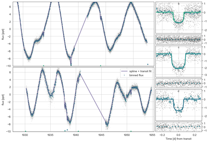
[11]:
mod.SampleModel(n_draws=1333)
mod.Plot(n_samp=101)
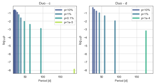
mod.PlotPeriods()
Multiprocess sampling (4 chains in 4 jobs)
NUTS: [phot_mean, logs2, u_star_tess, tdur_d, b_d, logror_d, t0_2_d, t0_d, tdur_c, b_c, logror_c, t0_2_c, t0_c, b_b, omega_b, ecc_b_frac, ecc_b_sigma_rayleigh, ecc_b_sigma_gauss, ecc_b, logror_b, per_b, t0_b, Rs, logrho_S]
Sampling 4 chains for 879 tune and 1_333 draw iterations (3_516 + 5_332 draws total) took 2207 seconds.
There was 1 divergence after tuning. Increase `target_accept` or reparameterize.
There was 1 divergence after tuning. Increase `target_accept` or reparameterize.
Saving sampled model parameters to file with shape: (246, 14)
When we have many possible aliases, we really want future photometry to be able to confirm them. You can generate a table of upcoming transits in MonoTools.fit using mod.PredictFutureTransits().
Here we ask for 50 days starting on March 7th (using astropy.Time)
[14]:
from astropy.time import Time
upcoming_trans = mod.PredictFutureTransits(time_start=Time('2022-03-07T00:00:00', format='isot', scale='utc'),
                                           time_dur=50)
upcoming_trans
time range 2022-03-07T00:00:00.000 -> 2022-04-25T19:49:50.292
[14]:
| transit_mid_date | transit_mid_med | transit_dur_med | transit_dur_-1sig | transit_dur_+1sig | transit_start_+2sig | transit_start_+1sig | transit_start_med | transit_start_-1sig | transit_start_-2sig | ... | transit_fractions | log_prob | prob | planet_name | alias_n | alias_p | aliases_ns | aliases_ps | total_prob | num_aliases | |
|---|---|---|---|---|---|---|---|---|---|---|---|---|---|---|---|---|---|---|---|---|---|
| 0 | 2022-03-08T13:25:28.308 | 2647.059355 | 0.176546 | 0.174889 | 0.178425 | 2646.983548 | 2646.977201 | 2646.971082 | 2646.964549 | 2646.957561 | ... | 19/4 | -16.192243 | 9.285353e-08 | duo_c | 3 | 47.282428 | 3,7 | 47.2824,23.6412 | 0.205571 | 2.0 |
| 1 | 2022-03-13T19:30:39.727 | 2652.312960 | 0.176546 | 0.174889 | 0.178425 | 2652.237219 | 2652.230838 | 2652.224687 | 2652.218118 | 2652.211088 | ... | 43/9 | -1.329252 | 2.646753e-01 | duo_c | 8 | 21.014413 | 8 | 21.0144 | 0.264675 | 1.0 |
| 2 | 2022-03-16T12:35:24.796 | 2655.024593 | 0.136204 | 0.134537 | 0.138170 | 2654.971464 | 2654.963541 | 2654.956490 | 2654.949625 | 2654.942411 | ... | 88 | 0.000000 | 1.000000e+00 | multi_b | 0 | 10.355724 | 0 | 10.3557 | 1.000000 | 1.0 |
| 3 | 2022-03-18T00:22:48.826 | 2656.515843 | 0.176546 | 0.174889 | 0.178425 | 2656.440156 | 2656.433747 | 2656.427570 | 2656.420972 | 2656.413910 | ... | 24/5 | -9.125435 | 1.088614e-04 | duo_c | 4 | 37.825943 | 4,9 | 37.8259,18.913 | 0.275734 | 2.0 |
| 4 | 2022-03-21T10:54:34.346 | 2659.954564 | 0.176546 | 0.174889 | 0.178425 | 2659.878922 | 2659.872493 | 2659.866291 | 2659.859671 | 2659.852582 | ... | 53/11 | -1.838018 | 1.591326e-01 | duo_c | 10 | 17.193610 | 10 | 17.1936 | 0.159133 | 1.0 |
| 5 | 2022-03-24T07:41:02.392 | 2662.820167 | 0.176546 | 0.174889 | 0.178425 | 2662.744561 | 2662.738116 | 2662.731893 | 2662.725251 | 2662.718142 | ... | 29/6 | -4.859221 | 7.756525e-03 | duo_c | 5 | 31.521619 | 5 | 31.5216 | 0.007757 | 1.0 |
| 6 | 2022-03-26T21:07:40.023 | 2665.380324 | 0.136204 | 0.134537 | 0.138170 | 2665.327362 | 2665.319342 | 2665.312222 | 2665.305277 | 2665.297971 | ... | 89 | 0.000000 | 1.000000e+00 | multi_b | 0 | 10.355724 | 0 | 10.3557 | 1.000000 | 1.0 |
| 7 | 2022-03-27T09:09:18.068 | 2665.881459 | 0.133908 | 0.129489 | 0.137680 | 2666.022889 | 2665.922736 | 2665.814505 | 2665.708043 | 2665.610466 | ... | 36/7 | -0.559529 | 5.714780e-01 | duo_d | 6 | 25.089347 | 6 | 25.0893 | 0.571478 | 1.0 |
| 8 | 2022-03-28T19:45:29.154 | 2667.323254 | 0.176546 | 0.174889 | 0.178425 | 2667.247708 | 2667.241236 | 2667.234981 | 2667.228306 | 2667.221165 | ... | 34/7 | -2.440342 | 8.713102e-02 | duo_c | 6 | 27.018530 | 6 | 27.0185 | 0.087131 | 1.0 |
| 9 | 2022-03-31T13:30:45.125 | 2670.063022 | 0.133908 | 0.129489 | 0.137680 | 2670.205592 | 2670.104908 | 2669.996068 | 2669.889008 | 2669.790883 | ... | 31/6 | -1.138605 | 3.202655e-01 | duo_d | 5 | 29.270905 | 5 | 29.2709 | 0.320265 | 1.0 |
| 10 | 2022-04-01T04:48:49.275 | 2670.700570 | 0.176546 | 0.174889 | 0.178425 | 2670.625069 | 2670.618577 | 2670.612297 | 2670.605597 | 2670.598433 | ... | 39/8 | -1.581966 | 2.055706e-01 | duo_c | 7 | 23.641214 | 7 | 23.6412 | 0.205571 | 1.0 |
| 11 | 2022-04-03T19:51:24.929 | 2673.327372 | 0.176546 | 0.174889 | 0.178425 | 2673.251905 | 2673.245397 | 2673.239099 | 2673.232379 | 2673.225196 | ... | 44/9 | -1.329252 | 2.646753e-01 | duo_c | 8 | 21.014413 | 8 | 21.0144 | 0.264675 | 1.0 |
| 12 | 2022-04-05T22:17:29.483 | 2675.428813 | 0.176546 | 0.174889 | 0.178425 | 2675.353375 | 2675.346853 | 2675.340540 | 2675.333806 | 2675.326607 | ... | 49/10 | -1.288714 | 2.756251e-01 | duo_c | 9 | 18.912971 | 9 | 18.913 | 0.275625 | 1.0 |
| 13 | 2022-04-06T05:39:54.607 | 2675.736049 | 0.136204 | 0.134537 | 0.138170 | 2675.683260 | 2675.675146 | 2675.667947 | 2675.660929 | 2675.653545 | ... | 90 | 0.000000 | 1.000000e+00 | multi_b | 0 | 10.355724 | 0 | 10.3557 | 1.000000 | 1.0 |
| 14 | 2022-04-06T10:00:47.004 | 2675.917211 | 0.133908 | 0.129489 | 0.137680 | 2676.061377 | 2675.959949 | 2675.850257 | 2675.742360 | 2675.643466 | ... | 26/5 | -2.252072 | 1.051810e-01 | duo_d | 4 | 35.125086 | 4 | 35.1251 | 0.105181 | 1.0 |
| 15 | 2022-04-07T15:33:22.300 | 2677.148175 | 0.176546 | 0.174889 | 0.178425 | 2677.072759 | 2677.066225 | 2677.059902 | 2677.053153 | 2677.045943 | ... | 54/11 | -1.838018 | 1.591326e-01 | duo_c | 10 | 17.193610 | 10 | 17.1936 | 0.159133 | 1.0 |
| 16 | 2022-04-15T04:45:49.823 | 2684.698493 | 0.133908 | 0.129489 | 0.137680 | 2684.845054 | 2684.742510 | 2684.631539 | 2684.522387 | 2684.422340 | ... | 21/4 | -5.784635 | 3.074434e-03 | duo_d | 3 | 43.906357 | 3 | 43.9064 | 0.003074 | 1.0 |
| 17 | 2022-04-16T14:12:09.132 | 2686.091772 | 0.136204 | 0.134537 | 0.138170 | 2686.039157 | 2686.030953 | 2686.023670 | 2686.016576 | 2686.009118 | ... | 91 | 0.000000 | 1.000000e+00 | multi_b | 0 | 10.355724 | 0 | 10.3557 | 1.000000 | 1.0 |
| 18 | 2022-04-21T11:17:59.255 | 2690.970825 | 0.133908 | 0.129489 | 0.137680 | 2691.119109 | 2691.015766 | 2690.903871 | 2690.793829 | 2690.692965 | ... | 37/7 | -0.559529 | 5.714780e-01 | duo_d | 6 | 25.089347 | 6 | 25.0893 | 0.571478 | 1.0 |
| 19 | 2022-04-24T20:12:11.274 | 2694.341797 | 0.176546 | 0.174889 | 0.178425 | 2694.266598 | 2694.259940 | 2694.253524 | 2694.246641 | 2694.239313 | ... | 5 | -85.995103 | 4.495739e-38 | duo_c | 0 | 189.129713 | 0,1,2,3,4,5,6,7,8,9,10,0,1,2,3,4,5,6 | 189.1297,94.5649,63.0432,47.2824,37.8259,31.52... | 2.000000 | 18.0 |
20 rows × 27 columns
If you want to directly export the predicted aliases to Cheops input XML files, with MonoTools you can with mod.MakeCheopsOR(). It’s necessary to specify which planet to generate
The Gaia DR2 ID must be specified, though if the lightcurve was loaded with lightcurve.multilc, then it’s pre-loaded from the TIC.
This has many things to tune, but the default produces at least 1 orbit on either side of the predicted transit (oot_min_orbits=1.0), covers the 3-sigma timing window (timing_sigma=3), includes a further 1.4 orbits of “flexibility” to assist in scheduling (orbits_flex=1.4), observes with minimum efficiency greater than 45% (min_eff=45), and will observe between 4 and 14 orbits (min_orbits=4.0,max_orbits=14).
In terms of which aliases, to schedule, MakeCheopsOR() produces ORs for the highest-probability aliases which together make up the 2-sigma period posterior (observe_sigma=2), observing the top-25% of these in priority 1 (prio_1_threshold=0.25), 0% in priority 3 (prio_3_threshold=0.0,) and the rest in priority 2 (i.e. 75%).
pycheops is necessary to finish the set-up of ORs using make_xml_files.
[16]:
c_cheops_ORs=mod.MakeCheopsOR(pl='c',observe_sigma=1.5,outfilesuffix='_example.csv')
c_cheops_ORs
INFO: Query finished. [astroquery.utils.tap.core]
time range 2022-01-27T14:03:42.476 -> 2022-07-26T14:03:42.476
Run the following command in a terminal to generate ORs:
"make_xml_files /Volumes/LUVOIR/MonoToolsData/TIC00027491137/TIC00027491137_2022-03-06_8_example.csv --auto-expose -f"
[16]:
| BJD_0 | BJD_early | BJD_late | Gaia_DR2 | Gmag | MinEffDur | N_Ranges | N_Visits | ObsReqName | Old_T_eff | ... | Priority | Programme_ID | SpTy | T_visit | Target | Vmag | _DEJ2000 | _RAJ2000 | e_Gmag | e_Vmag | |
|---|---|---|---|---|---|---|---|---|---|---|---|---|---|---|---|---|---|---|---|---|---|
| 7 | 2.458938e+06 | 2.459607e+06 | 2.459787e+06 | 1490845584382687232 | 8.910282 | 45 | 0 | 1 | TIC27491137_c_period23;64_prob0.20 | -99.0 | ... | 2 | 0048 | K1 | 35402 | TIC27491137 | 9.121931 | 39:47:25.545 | 14:29:34.2428 | 0.000479 | 0.046337 |
| 8 | 2.458938e+06 | 2.459607e+06 | 2.459787e+06 | 1490845584382687232 | 8.910282 | 45 | 0 | 1 | TIC27491137_c_period21;01_prob0.26 | -99.0 | ... | 2 | 0048 | K1 | 35402 | TIC27491137 | 9.121931 | 39:47:25.545 | 14:29:34.2428 | 0.000479 | 0.046337 |
| 9 | 2.458938e+06 | 2.459607e+06 | 2.459787e+06 | 1490845584382687232 | 8.910282 | 45 | 0 | 1 | TIC27491137_c_period18;91_prob0.27 | -99.0 | ... | 2 | 0048 | K1 | 35402 | TIC27491137 | 9.121931 | 39:47:25.545 | 14:29:34.2428 | 0.000479 | 0.046337 |
3 rows × 23 columns
Using MonoTools.fit on a real Duotransit with RVs
We can also use radial velocities to instruct our Duotransit fits.
Let’s use the TOI-561 system as an example, for which the RVs were published in Lacedelli 2022.
Unfortunately, the way it is currently implemented, including RVs in MonoTools.fit only works with a single duo or monotransiting planet… So we will assume the 24d planet is solved (at is was with e.g. Cheops) and only the outer planet has an undetermined period.
To include the RVs, we need to call the add_rvs function with a dictionary loaded with array of time, rv, rv_err, plus extra info on the rv_unit (kms or ms), the time zero point jd_base, and potentially a telescope index array (with strings associating each RV with each telescope).
[2]:
toi561 = fit.monoModel(377064495,'tess')
Getting all IDs
Empty TableList
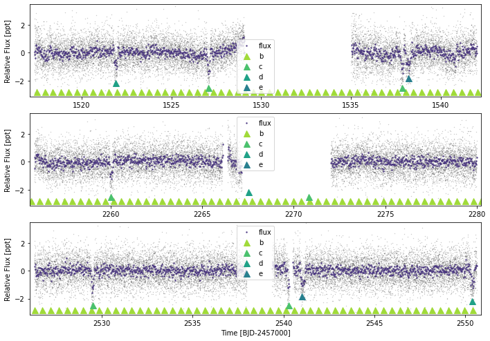
Let’s plot the true ephemeridis:
[3]:
toi561.lc.plot(plot_ephem={'b':{'p':0.4465688,'period_err':0.000001,'t0':2317.7498,'tdur':1.31/24,'depth':0.0155**0.5},
                           'c':{'p':10.778831,'period_err':0.000036,'t0':2238.4629,'tdur':3.75/24,'depth':0.0316**0.5},
                           'd':{'p':25.7124,'period_err':0.0001,'t0':2318.966,'tdur':4.54/24,'depth':0.0306**0.5},
                           'e':{'p':77.14,'period_err':0.25,'t0':1538.180,'tdur':6.98/24,'depth':0.0278**0.5}})
[4]:
from MonoTools import tools
from astropy.io import ascii
init_rv_tab=ascii.read(tools.MonoData_tablepath+'/TOI561_table2.dat').to_pandas()
rvtab={'time':init_rv_tab['BJD_TDB'].values-2457000,
       'rv':init_rv_tab['RV'].values,
       'rv_err':init_rv_tab['err_RV'].values,
       'rv_unit':'m/s'}
Including the RVs and stellar parameters from Lacedelli et al
using add_rvs and init_starpars.
We can specify the degree of polynomial trend we want to include in the RV fitting using n_poly_trend (default is 2).
[5]:
toi561.add_rvs(rvtab,n_poly_trend=2)
Assuming RV unit is in m/s
Assuming all one telescope (HARPS).
[6]:
toi561.init_starpars(Rstar=[0.843,0.005,0.005],
                     logg=[4.5,0.12,0.12],
                     Mstar=[0.806,0.12,0.036],
                     Teff=[5372,70,70])
Initialising the four planets and model:
[7]:
toi561.add_planet('multi',{'period':0.4465688,'period_err':0.000001,'tcen':2317.7498,'tdur':1.31/24,'depth':0.0155**2,'K':1.56},'b')
toi561.add_planet('multi',{'period':10.778831,'period_err':0.000036,'tcen':2238.4629,'tdur':3.75/24,'depth':0.0316**2,'K':1.84},'c')
toi561.add_planet('multi',{'period':25.7124,'period_err':0.0001,'tcen':2318.966,'tdur':4.54/24,'depth':0.0306**2,'K':3.1},'d')
toi561.add_planet('duo',{'tcen':1538.180,'tcen_2':2541.08,'tdur':6.98/24,'depth':0.0278**2},'e')
[10]:
toi561.init_model(use_GP=False,
                  bin_oot=False,
                  cut_distance=1.75)
rv_offsets __str__ = [79699.73]
logK __str__ = 0.44468582126144574
logK __str__ = 0.6097655716208943
logK __str__ = 1.1314021114911006
min_eccs[pl] __str__ = [0.70507819 0.56915964 0.47082042 0.39290426 0.32823486 0.27297434
 0.22478612 0.18212606 0.14391373 0.1093605  0.07787159 0.04898653
 0.02234115 0.00235778 0.04683396 0.06697604 0.12065873 0.13665255
 0.15183626 0.18003928 0.20572586 0.21774181 0.22925865 0.26114276
 0.28045379 0.29842345 0.31520244 0.36623555]
omegas[pl] __str__ = [1.57079633 1.57079633 1.57079633 1.57079633 1.57079633 1.57079633
 1.57079633 1.57079633 1.57079633 1.57079633 1.57079633 1.57079633
 1.57079633 4.71238898 4.71238898 4.71238898 4.71238898 4.71238898
 4.71238898 4.71238898 4.71238898 4.71238898 4.71238898 4.71238898
 4.71238898 4.71238898 4.71238898 4.71238898]
bs[pl] __str__ = 0.1
t0s[pl] __str__ = 2541.08
pers[pl] __str__ = [1002.9         501.45        334.3         250.725       200.58
  167.15        143.27142857  125.3625      111.43333333  100.29
   91.17272727   83.575        77.14615385   71.63571429   62.68125
   58.99411765   50.145        47.75714286   45.58636364   41.7875
   38.57307692   37.14444444   35.81785714   32.3516129    30.39090909
   28.65428571   27.10540541   22.79318182]
sum_normalised_rvs __str__ = [15.9315571  32.99435949 81.5296839  73.89434729 70.82593254 78.12525271
 63.00798691 62.79199858 64.43329749 79.15791019 77.59827531 67.64188314
 76.27142951 71.22409354 51.49071752 68.12045065 75.84031138 64.74834132
 87.09292796 82.93901425 69.30972683 85.61268135 67.88859309 72.2715288
 83.12708244 58.81131763 70.02639181 77.79229431]
nonmarg_rvs __str__ = [79701.15913667 79701.66097252 79701.87720865 79700.40916249
 79699.03635222 79697.98538911 79699.75731766 79699.33217773
 79702.21435266 79698.64069765 79700.29288086 79697.56277972
 79699.12573312 79699.8236008  79698.4665334  79702.76133202
 79703.29438918 79700.96392605 79700.9517529  79705.07587114
 79704.8910157  79701.03362767 79701.9480563  79700.07787419
 79698.21158538 79699.46952654 79700.27518367 79699.56362595
 79698.95578653 79698.11862623 79698.00751118 79697.53472773
 79697.15563034 79697.08720977 79697.02713144 79697.05825177
 79697.37673831 79697.60378114 79699.09836702 79700.79931169
 79704.13272783 79699.86300919 79698.72495703 79698.46238598
 79698.32924137 79698.33416148 79697.89114593 79697.87085205
 79698.09420697 79698.96298941 79701.52300435 79699.97362522
 79698.94759079 79697.75131774 79696.64608613 79697.11073235
 79696.97036768 79698.96761918 79698.51287062 79697.71304074
 79699.1927153  79697.10657679 79697.37600681 79698.42721894
 79702.02211131 79702.1766203  79701.78514832 79703.90677921
 79701.45891715 79701.65083861 79698.47839524 79699.09625045
 79701.52845064 79700.69661958 79696.95930088 79697.41500963
 79699.5350849  79699.02375907 79704.34026451 79703.04588714
 79702.09842602 79697.808998   79697.33318103 79699.19099681
 79700.27362581 79698.65186119 79702.22256108 79703.76353998
 79702.90048169 79703.70828588 79696.67400631 79696.67583912
 79696.7131976  79696.81144399 79696.9442293  79697.14914408
 79697.45081015 79697.93237746 79697.05855757 79698.16704259
 79699.02532054 79698.4167408  79698.04637662 79697.81085946
 79697.65995274 79697.55821502 79700.86112607 79701.32804173
 79701.6238418  79699.58524974 79696.6254821  79696.69130106
 79698.26464947 79697.89282371 79697.20800003 79697.90846243
 79698.27638982 79702.3189119  79705.60629515 79700.52758787
 79697.88849409 79697.17309899 79698.41140933 79700.9951051
 79697.894082   79697.40304076 79697.04766657 79696.89700502
 79700.38963984 79697.93180748 79697.05223853 79696.84850617
 79703.04161115 79702.45522508 79703.49898362 79703.4838004
 79699.83935276 79697.01247462 79698.40081866 79698.35879808
 79699.23973915 79701.77835291 79706.31093183 79705.36639126]
self.rvs['rv'] - nonmarg_rvs __str__ = [-5.18913667 -2.00097252 -4.37720865 -4.82916249  2.20364778  4.48461089
  1.75268234  3.23782227  0.66564734 -1.81069765 -0.92288086  1.20722028
  4.40426688  3.8163992   3.7734666  -2.11133202 -4.84438918 -5.44392605
 -4.0817529  -6.91587114 -6.9010157  -7.54362767 -3.4780563  -8.30787419
 -4.46158538 -0.98952654 -1.95518367 -3.17362595 -6.21578653 -2.99862623
 -6.24751118 -3.68472773 -3.11563034 -1.86720977 -1.53713144 -0.77825177
 -0.26673831  3.62621886  1.95163298  4.39068831 -5.06272783 -2.28300919
  0.64504297  1.71761402 -1.26924137  1.39583852 -1.14114593  2.84914795
  0.48579303  2.12701059 -2.28300435 -1.87362522  0.28240921 -1.27131774
  5.55391387  7.60926765  6.82963232  5.76238082  7.00712938  7.66695926
  5.7772847   9.17342321  9.97399319 13.86278106  6.58788869  3.2033797
  7.41485168  0.27322079  1.65108285  2.25916139  2.99160476  5.98374955
  5.42154936 -0.07661958 -0.32930088 -0.68500963  8.8249151   6.84624093
  0.17973549 -3.35588714  0.46157398  0.161002   -1.95318103  0.53900319
 -7.72362581  8.81813881  6.07743892  0.37646002 -1.14048169 -8.79828588
 -2.75400631  0.30416088  0.3268024  -1.74144399  0.0457707   1.08085592
  2.82918985  1.32762254  4.61144243  3.92295741  2.35467946 -0.6467408
  2.01362338  1.44914054  2.67004726  1.07178498  2.30887393  3.67195827
  1.5261582  -3.50524974 -3.5054821   1.40869894  0.49535053  2.35717629
 -1.71800003  2.80153757  5.41361018  4.8210881  -0.98629515 -4.43758787
 -1.74849409  0.76690101  1.91859067  0.0248949  -2.464082   -1.03304076
  3.30233343  4.35299498 -6.25963984 -7.65180748 -3.49223853 -3.72850617
  5.79838885 -0.34522508  3.56101638 -5.5038004  -3.12935276  6.30752538
  4.96918134  5.00120192  4.37026085  4.75164709 -0.96093183 -3.31639126]
tt.tile(self.rvs['rv'] - nonmarg_rvs,(self.n_margs[pl],1)) __str__ = [[-5.18913667 -2.00097252 -4.37720865 ...  4.75164709 -0.96093183
  -3.31639126]
 [-5.18913667 -2.00097252 -4.37720865 ...  4.75164709 -0.96093183
  -3.31639126]
 [-5.18913667 -2.00097252 -4.37720865 ...  4.75164709 -0.96093183
  -3.31639126]
 ...
 [-5.18913667 -2.00097252 -4.37720865 ...  4.75164709 -0.96093183
  -3.31639126]
 [-5.18913667 -2.00097252 -4.37720865 ...  4.75164709 -0.96093183
  -3.31639126]
 [-5.18913667 -2.00097252 -4.37720865 ...  4.75164709 -0.96093183
  -3.31639126]]
normalised_rv_models[pl].T __str__ = [[-0.39239524 -0.39026662 -0.38829365 ...  0.60066443  0.6033578
   0.60599904]
 [ 0.06620089  0.0706856   0.07485507 ...  0.32277676  0.32734611
   0.33181906]
 [ 0.80669786  0.8156726   0.82396841 ... -0.06534405 -0.05762688
  -0.05009168]
 ...
 [-0.96137196 -0.99941045 -0.97360183 ...  0.46150028  0.33890444
   0.21787972]
 [ 0.57041446  0.43806283  0.313144   ...  0.2380481   0.63385618
   0.8769599 ]
 [ 0.92706664  0.8075466   0.67858538 ... -0.8950983  -0.98100433
  -0.99132386]]
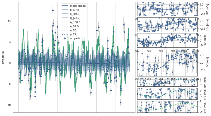
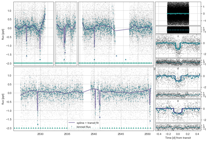
Plotting the photometric and RV models:
[11]:
toi561.Plot()
initialising transit
Initalising Transit models for plotting with n_samp= 10

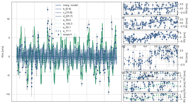
Here, the RVs plot the timeseries on the left and the phase-folds on the right.
The upper three RV vurves correspond to the multi-transiting planets, while the lower four phase-folded RV curves with dashed lines correspond to the best-fitting period aliases from the model.
Similarly, the dashed lines on the right show the best-fit RV models for the best period aliases, though the transparency of these are weighted by probability, and in this case only the 77.1d alias appears present (as it shows by far the strongest RV signal).
[12]:
toi561.PlotRVs()
Sampling the TOI-561 model
This is a big model so we haven’t included enough samples here for a reasonable result yet, but this should be demonstrative.
[13]:
toi561.SampleModel(n_samp=250)
Multiprocess sampling (4 chains in 4 jobs)
NUTS: [phot_mean, rv_logs2, rv_polys, rv_offsets, logs2, u_star_tess, tdur_e, b_e, logror_e, t0_2_e, t0_e, logK_d, b_d, omega_d, ecc_d_frac, ecc_d_sigma_rayleigh, ecc_d_sigma_gauss, ecc_d, logror_d, per_d, t0_d, logK_c, b_c, omega_c, ecc_c_frac, ecc_c_sigma_rayleigh, ecc_c_sigma_gauss, ecc_c, logror_c, per_c, t0_c, logK_b, b_b, omega_b, ecc_b_frac, ecc_b_sigma_rayleigh, ecc_b_sigma_gauss, ecc_b, logror_b, per_b, t0_b, Rs, logrho_S]
Sampling 4 chains for 330 tune and 500 draw iterations (1_320 + 2_000 draws total) took 687 seconds.
The acceptance probability does not match the target. It is 0.9666844230354691, but should be close to 0.9. Try to increase the number of tuning steps.
The acceptance probability does not match the target. It is 0.9742654142610762, but should be close to 0.9. Try to increase the number of tuning steps.
Saving sampled model parameters to file with shape: (536, 14)
[14]:
toi561.Plot()
[15]:
toi561.PlotRVs()
[17]:
toi561.PlotPeriods(xlog=True,ymin=-20)
Here we can see that the model with photometry + RVs clearly found the 77d period, with a preference of \(\sim1\times10^{12}\) over the next-closest RV aliases.
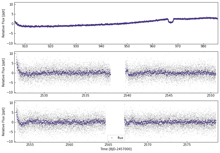
Let’s revisit EPIC248847494 - a 54hour-long transit event seen in K2.
Previously, we used a circular orbital fit and predicted a planet with a 3650d orbit!
[2]:
k2=fit.monoModel(248847494,'k2')
Getting all IDs
INFO  [everest.user.DownloadFile()]: Found cached file.
INFO  [everest.user.load_fits()]: Loading FITS file for 248847494.
[3]:
k2.lc.plot()
32526
Adding the stellar parameters from Giles et al (2019):
[4]:
k2.init_starpars(Rstar=[2.70,0.12,0.12],Mstar=[0.9,0.09,0.09],Teff=[4898,68,68])
Adding the mono-transit candidate:
One problem with this transit is that it is SO long… Given our strong period prior (shorter orbits are vastly preferred), this actually means the model tries its best to shorten the orbit and therefore transit, jeapordising the fit. So we need to make sure that this isn’t the case by including en error on the transit duation.
We also cannot use a GP, as this tends to try to fit away the transit.
[5]:
k2.add_mono({'tcen':967.17,'tdur':53.6/24,'tdur_err':1.5/24,'depth':0.045**2},'b')
[51]:
k2.init_model(use_GP=False,bin_oot=False)
[52]:
k2.SampleModel()
[64]:
df=k2.MakeTable()
df
Saving sampled model parameters to file with shape: (573, 14)
[64]:
| mean | sd | hdi_3% | hdi_97% | mcse_mean | mcse_sd | ess_bulk | ess_tail | r_hat | 5% | -$1\sigma$ | median | +$1\sigma$ | 95% | |
|---|---|---|---|---|---|---|---|---|---|---|---|---|---|---|
| Rs[0] | 2.75132 | 0.65406 | 1.37806 | 3.83070 | 0.03768 | 0.02777 | 336.59789 | 89.64571 | 1.27154 | 1.74281 | 2.23275 | 2.68592 | 3.24933 | 3.89824 |
| logs2[0] | -3.97720 | 0.14379 | -4.22246 | -3.67007 | 0.00927 | 0.00656 | 263.76602 | 125.69915 | 1.23816 | -4.16491 | -4.07907 | -3.99850 | -3.88258 | -3.68851 |
| logs2[1] | -1.78759 | 0.38781 | -2.46612 | -1.10929 | 0.04267 | 0.03636 | 242.54078 | 52.61684 | 1.07372 | -2.40559 | -2.06146 | -1.75149 | -1.47502 | -1.28733 |
| phot_mean | 0.00137 | 0.01642 | -0.02904 | 0.03386 | 0.00054 | 0.00175 | 617.81789 | 34.72315 | 1.25616 | -0.02112 | -0.00668 | 0.00261 | 0.01016 | 0.01905 |
| rho_S | 0.67776 | 2.58243 | 0.00268 | 2.42730 | 0.26495 | 0.18793 | 212.77798 | 99.35770 | 1.08226 | 0.00415 | 0.00799 | 0.03434 | 0.31874 | 3.22334 |
| ... | ... | ... | ... | ... | ... | ... | ... | ... | ... | ... | ... | ... | ... | ... |
| logprob_b[45] | -12.52269 | 3.03808 | -17.46260 | -7.86351 | 0.70581 | 0.51991 | 21.78087 | 309.85763 | 1.12843 | -17.49988 | -16.10002 | -11.84795 | -9.44810 | -8.51475 |
| ecc_b | 0.52597 | 0.36112 | 0.00000 | 0.92085 | 0.06400 | 0.04568 | 59.42654 | 368.15204 | 1.06395 | 0.00000 | 0.00000 | 0.68625 | 0.88475 | 0.92591 |
| ecc_marg_b | 0.52597 | 0.36112 | 0.00000 | 0.92085 | 0.06400 | 0.04568 | 59.42654 | 368.15204 | 1.06394 | 0.00000 | 0.00000 | 0.68625 | 0.88475 | 0.92591 |
| vel_marg_b | 0.44220 | 0.27760 | 0.10074 | 1.06475 | 0.01680 | 0.01396 | 300.32200 | 84.17450 | 1.10880 | 0.09450 | 0.17773 | 0.37724 | 0.75923 | 1.02706 |
| per_marg_b | 145.16052 | 70.99660 | 76.26878 | 286.32924 | 3.11964 | 2.20716 | 432.50262 | 322.17440 | 1.07679 | 84.97405 | 114.78203 | 122.27528 | 168.72628 | 311.19314 |
573 rows × 14 columns
[86]:
np.unique([i.split("[")[0] for i in df.index])
[86]:
array(['Ms', 'Rs', 'a_Rs_b', 'b_b', 'ecc_b', 'ecc_marg_b',
       'gap_width_prior_b', 'logmassest_b', 'logprior_b', 'logprob_b',
       'logror_b', 'logs2', 'logvel_b', 'max_ecc_b', 'min_ecc_b',
       'omega_b', 'per_b', 'per_marg_b', 'per_prior_b', 'phot_mean',
       'rho_S', 'ror_b', 'rpl_b', 't0_b', 'tdur_b', 'u_star_kep',
       'u_star_tess', 'v_prior_b', 'vel_b', 'vel_marg_b'], dtype='<U17')
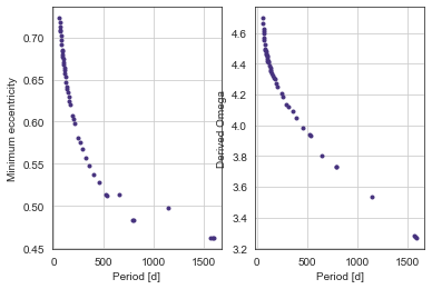
Interestingly, the model prefers high-eccentricity, short-period gaps over low-eccentricity low-period gaps.
i.e. the Period prior wins out over the eccentricity prior.
In this case too - the derived marginalised argument of periastron is ~1.5pi in the high-eccentricity case, showing that these orbits favour a transit at apohelion (again, the opposite of what we expect from purely geometrical transit probability).
[89]:
plt.subplot(121)
plt.plot([df.loc['per_b['+str(nper)+']','mean'] for nper in range(45)],
         [df.loc['min_ecc_b['+str(nper)+']','mean'] for nper in range(45)],'.')
plt.xlabel("Period [d]")
plt.ylabel("Minimum eccentricity")

plt.subplot(122)
plt.plot([df.loc['per_b['+str(nper)+']','mean'] for nper in range(45)],
         [df.loc['omega_b['+str(nper)+']','mean'] for nper in range(45)],'.')
plt.xlabel("Period [d]")
plt.ylabel("Derived Omega")
[89]:
Text(0, 0.5, 'Derived Omega')
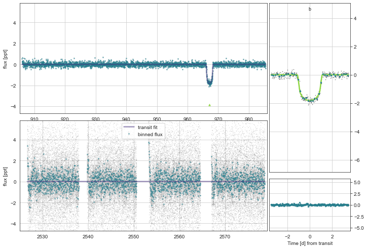
[54]:
k2.Plot(plot_flat=True,n_samp=150)
32526
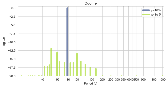
Here is the period vs probability distribution.
The gaps in the TESS lightcurve are causing some bizarre phantom-peaks that I am investigating, but the effect is the same - shorter-period solutions are favoured.
[63]:
k2.PlotPeriods(xlog=True,pmin=55,pmax=1240,ymin=1e-8)
1e-08 1.0
1e-08 None True
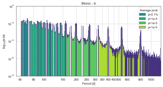
Here the marginalised period is \(145\pm71\) days (90% region from 85 to 310d) - far lower than the circular orbit derived in Giles et al (2019)
[92]:
print(df.loc['per_marg_b'])
mean          145.16052
sd             70.99660
hdi_3%         76.26878
hdi_97%       286.32924
mcse_mean       3.11964
mcse_sd         2.20716
ess_bulk      432.50262
ess_tail      322.17440
r_hat           1.07679
5%             84.97405
-$1\sigma$    114.78203
median        122.27528
+$1\sigma$    168.72628
95%           311.19314
Name: per_marg_b, dtype: float64