Using MonoTools.lightcurve

The fit and search modules take in, as default, lightcurve.lc objects. Here we’ll give a very quick overview of how to use them.

The simplest way to use a lightcurve object, is simply to load externally your data, and make a lightcurve object from them, by passing time, flux and flux_err arrays.

First let’s import the module and other useful stuff:

%load_ext autoreload
%autoreload 2
from MonoTools import lightcurve as lc
import numpy as np
import matplotlib.pyplot as plt
%matplotlib inline

/Users/hosborn/miniconda3/envs/newxo/lib/python3.9/site-packages/theano/configparser.py:255: UserWarning: Theano does not recognise this flag: gcc.cxxflags
  warnings.warn(f"Theano does not recognise this flag: {key}")
Matplotlib created a temporary config/cache directory at /var/folders/p0/tmr0j01x4jb3qrbc5b0gnxcw0000gn/T/matplotlib-hmgdrkv4 because the default path (/Users/hosborn/.matplotlib) is not a writable directory; it is highly recommended to set the MPLCONFIGDIR environment variable to a writable directory, in particular to speed up the import of Matplotlib and to better support multiprocessing.

Loading a TESS, K2 or Kepler lightcurve

The easiest way to use MonoTools.lightcurve is to not bother with the load_lc function defined below, but instead to jump straight to extracting a multilc class from a search of Kepler, K2 and TESS data.

This is possible simply by passing an id and mission argument to the multilc class.

It will search the given mission, but if do_search is True, it will also search other missions for corresponding data using the multilc.get_all_lightcurves() function. This function is assisted by including a radec in astropy.coordinates.SkyCoord format as an argument when initialising the multilc class (as otherwise, we have to access the input catalogue and then use the ra & dec to search for extra data).

Set load=False if you do not want to load from file.

TESS Example: Nu2 Lupi

tesslc=lc.multilc(136916387, 'tess')

Getting all IDs
Accessing online catalogues to match ID to RA/Dec (may be slow) mission= tess
          ID         ra        dec     pmRA    pmDEC    Tmag objType  typeSrc  \
0  136916387  230.45063 -48.317628 -1624.05 -276.024  5.0494    STAR  tmgaia2

    version    HIP  ... splists      e_RA     e_Dec     RA_orig   Dec_orig  \
0  20190415  75181  ...     NaN  2.864235  2.064396  230.440115 -48.318817

  e_RA_orig e_Dec_orig raddflag wdflag  dstArcSec
0  0.068131   0.057039        1      0        0.0

[1 rows x 125 columns]
Empty TableList
Sector 48 not (yet) found on MAST | RESPONCE:404
Sector 49 not (yet) found on MAST | RESPONCE:404

If other missions have been searched, the info should end up in multilc.all_ids.

You can see that the TESS input catalog has been searched and stored at tesslc.all_ids['tess']['data'], which is useful.

#In this case there are no extra lightcurves from e.g. Kepler, K2 or CoRoT:
tesslc.all_ids

{'tess': {'id': 136916387,
  'data': ID            136916387
  ra            230.45063
  dec          -48.317628
  pmRA           -1624.05
  pmDEC          -276.024
                  ...
  e_RA_orig      0.068131
  e_Dec_orig     0.057039
  raddflag              1
  wdflag                0
  dstArcSec           0.0
  Name: 0, Length: 125, dtype: object,
  'search': [12, 38]},
 'k2': {},
 'kepler': {},
 'corot': {}}

Plotting

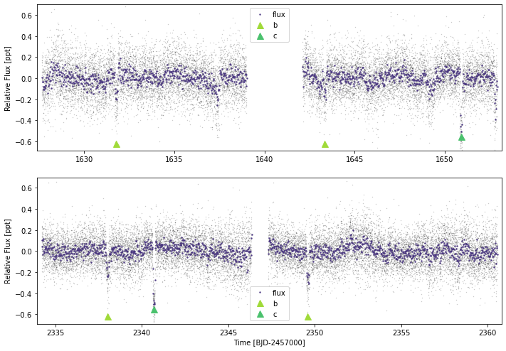
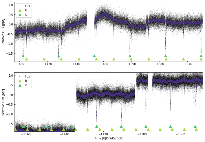
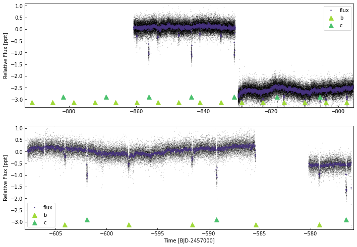
Now you have a lightcurve, then you can plot using lc.plot(). For high-cadence data (<30 minutes), it will perform binning and plot these are stronger points.

Useful arguments include: - plot_rows How many rows would you like to split the data over? - timeseries: If you want to plot more than just flux, then include those timeseries here (e.g. bg_flux, raw_flux, flux_flat etc). These other timeseries can be offset using the y_offset argument - ylim and xlim: If you don’t want to plot the whole x or y span, then cut them here. - plot_ephem: You can easily mark where the transits of planets are by including a dictionary in the form plot_ephem={'planet_name':{'p':10.0,'t0':2300.0,'tdur':0.4}}. Transits are then marked with triangles

tesslc.plot(plot_rows=2,plot_ephem={'b':{'p':11.57797,'t0':1944.3726,'tdur':3.9/24},
                                    'c':{'p':27.59221,'t0':1954.4099,'tdur':3.2/24}})

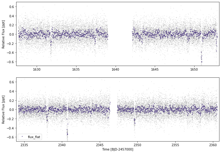
tesslc.flatten(knot_dist=0.6,ephems={'b':{'p':11.57797,'t0':1944.3726,'tdur':3.9/24},
                                    'c':{'p':27.59221,'t0':1954.4099,'tdur':3.2/24}})
tesslc.plot(timeseries=['flux_flat'])

TESS + K2 Example - K2-167

As the lightcurve module cross-checked with other catalogues, it needs and RA & Dec, so unless you specify an RA & Dec along with the initialisation, it goes searching for one from the input catalogue (which can be slow).

from astropy.coordinates import SkyCoord,FK5
from astropy import units as u

k2lc=lc.multilc(248777106,'k2',radec=SkyCoord("10h18m41.06s +10d07m43.85s",unit=(u.hourangle,u.deg)))

Getting all IDs
DEBUG [urllib3.connectionpool._new_conn()]: Starting new HTTPS connection (1): exofop.ipac.caltech.edu:443
DEBUG [urllib3.connectionpool._make_request()]: https://exofop.ipac.caltech.edu:443 "GET /k2/download_target.php?id=248777106 HTTP/1.1" 200 6893
DEBUG [urllib3.connectionpool._new_conn()]: Starting new HTTPS connection (1): mast.stsci.edu:443
DEBUG [urllib3.connectionpool._make_request()]: https://mast.stsci.edu:443 "GET /api/v0/invoke?request=%7B%22service%22%3A%20%22Mast.Name.Lookup%22%2C%20%22params%22%3A%20%7B%22input%22%3A%20%22EPIC%20248777106%22%2C%20%22format%22%3A%20%22json%22%7D%7D HTTP/1.1" 200 None
DEBUG [urllib3.connectionpool._make_request()]: https://mast.stsci.edu:443 "POST /api/v0/invoke HTTP/1.1" 200 None
DEBUG [urllib3.connectionpool._make_request()]: https://mast.stsci.edu:443 "POST /api/v0/invoke HTTP/1.1" 200 None
Sector 48 not (yet) found on MAST | RESPONCE:404
Sector 49 not (yet) found on MAST | RESPONCE:404
INFO  [everest.user.DownloadFile()]: Found cached file.
INFO  [everest.user.load_fits()]: Loading FITS file for 248777106.

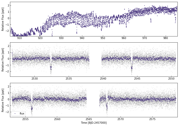
We can see which sectors/campaigns (and with which detrending) are loaded using the cadence_list:

k2lc.cadence_list

['ts_120_pdc_45', 'ts_120_pdc_46', 'k2_1800_ev_14']

k2lc.plot()

TESS + Kepler Example - Kepler-25

Once again, we need the KIC (4349452 in this case).

Accessing Kepler data can take a bit more time (as there’s 4-years worth!).

keplc=lc.multilc(4349452,'kepler')

Getting all IDs
DEBUG [urllib3.connectionpool._new_conn()]: Starting new HTTP connection (1): vizier.u-strasbg.fr:80
DEBUG [urllib3.connectionpool._make_request()]: http://vizier.u-strasbg.fr:80 "POST /viz-bin/votable HTTP/1.1" 200 660
DEBUG [urllib3.connectionpool._new_conn()]: Starting new HTTP connection (1): vizier.u-strasbg.fr:80
DEBUG [urllib3.connectionpool._make_request()]: http://vizier.u-strasbg.fr:80 "POST /viz-bin/votable HTTP/1.1" 200 689

keplc.cadence_list

['ts_120_pdc_14',
 'ts_120_pdc_40',
 'ts_120_pdc_41',
 'k1_1800_pdc_0',
 'k1_1800_pdc_1',
 'k1_59_pdc_2',
 'k1_1800_pdc_3',
 'k1_1800_pdc_4',
 'k1_59_pdc_5',
 'k1_59_pdc_6',
 'k1_59_pdc_7',
 'k1_59_pdc_8',
 'k1_59_pdc_9',
 'k1_59_pdc_10',
 'k1_59_pdc_11',
 'k1_59_pdc_12',
 'k1_59_pdc_13',
 'k1_59_pdc_14',
 'k1_59_pdc_15',
 'k1_59_pdc_16',
 'k1_59_pdc_17']

5703.42004-7000

-1296.57996

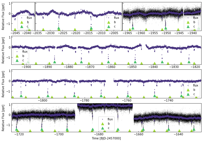
Given all this data, plotting will also take some time…

keplc.plot(plot_ephem={'b':{'p':6.2385,'t0':5703.42004-7000,'tdur':0.1},
                            'c':{'p':12.7204,'t0':5711.15013-7000,'dur':0.15}},
           cadences=['k1_1800_pdc_0', 'k1_1800_pdc_1', 'k1_59_pdc_2', 'k1_1800_pdc_3', 'k1_1800_pdc_4', 'k1_59_pdc_5'])

keplc.plot(plot_ephem={'b':{'p':6.2385,'t0':5703.42004-7000,'tdur':0.1},
                       'c':{'p':12.7204,'t0':5711.15013-7000,'dur':0.15}},
           cadences=['k1_1800_pdc_6', 'k1_1800_pdc_7', 'k1_59_pdc_8', 'k1_1800_pdc_9', 'k1_1800_pdc_10', 'k1_59_pdc_11'])

keplc.plot(plot_ephem={'b':{'p':6.2385,'t0':5703.42004-7000,'tdur':0.1},
                       'c':{'p':12.7204,'t0':5711.15013-7000,'dur':0.15}},
           cadences=['k1_1800_pdc_12', 'k1_1800_pdc_13', 'k1_59_pdc_14', 'k1_1800_pdc_15', 'k1_1800_pdc_16', 'k1_59_pdc_17'],)

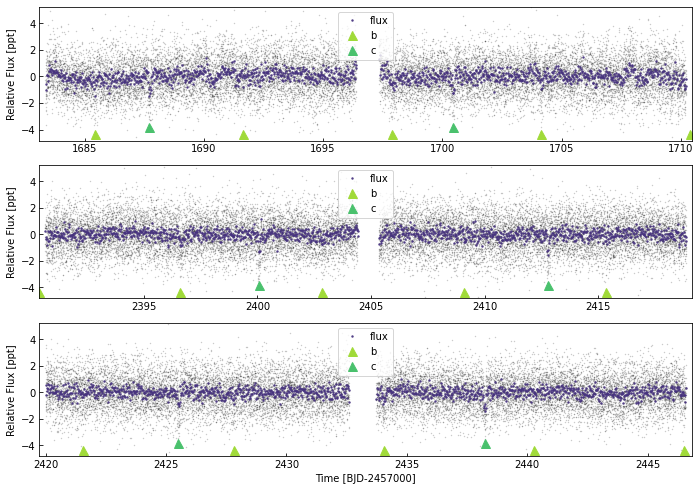
keplc.plot(plot_ephem={'b':{'p':6.2385,'t0':5703.42004-7000,'tdur':0.1},
                       'c':{'p':12.7204,'t0':5711.15013-7000,'dur':0.15}},
           cadences=['ts_120_pdc_14', 'ts_120_pdc_40', 'ts_120_pdc_41'])

Creating an interactive plot:

We can also create an interactivet plot using the command interactive_plot. This creates a bokeh stand-alone html page:

tesslc.interactive_plot(timeseries=['flux','flux_flat'],yoffset=0.8, plot_height=900,overwrite=True,ylim=(-1,2),
                        plot_ephem={'b':{'p':11.57797,'t0':1944.3726,'tdur':3.9/24},
                                    'c':{'p':27.59221,'t0':1954.4099,'tdur':3.2/24}})

binning: ['flux', 'flux_flat']
[nan, nan, nan, 0.0062, 0.0914699, nan, nan, 0.021, 0.03, 0.226, 0.0015675, 110.683, 0.0756251, 0.1, 0.0451056, 0.127035, 0.189496, 0.01985]

Initialising a simple lightcurve from pre-loaded data

The above lightcurve methods create a MonoTools.lightcurve.multilc method. But this inherits the base MonoTools.lightcurve.lc class and is built from combinations of individual lc objects.

The base class MonoTools.lightcurve.lc can also be simply loaded using time/flux/flux_err arrays.

Here’s some important info for calling lc.load_lc().

You must specify the “flux system” underlying the lightcurve flux - ppm: normalised lightcurve with median at 0.0 with units in parts per million - ppt: normalised lightcurve with median at 0.0 with units in parts per thousand (this is the default) - norm0: normalised lightcurve with median at 0.0 with units as a ratio (0->1) - norm1: normalised lightcurve with median at 1.0 with units as a ratio (0->1) - elec: un-normalised lightcurve with units of pure electrons where the median is proportional to stellar magnitude

The flux system can be changed using lc.change_flux_system(new_flx_system) (and is automatically made uniform when stacking lc objects).

As with flx_system, we need to know the base system used for the lightcurve time. The default is the TESS system using jd_base=2457000

The arguments identify the source of the lightcurve, and are necessary if you plan to stack multiple lightcurves together. - mission: the photometric mission providing the lightcurve in lowercase (e.g. k2, tess, kepler, etc) - sect: the sector, campaign or quarter within that mission the data comes from - src: a identifier for the source of the lightcurve detrending. e.g. pdc (most kepler quarters), vand, ev or pdc (for k2 campaigns), pdc, qlp or el (for tess sectors)

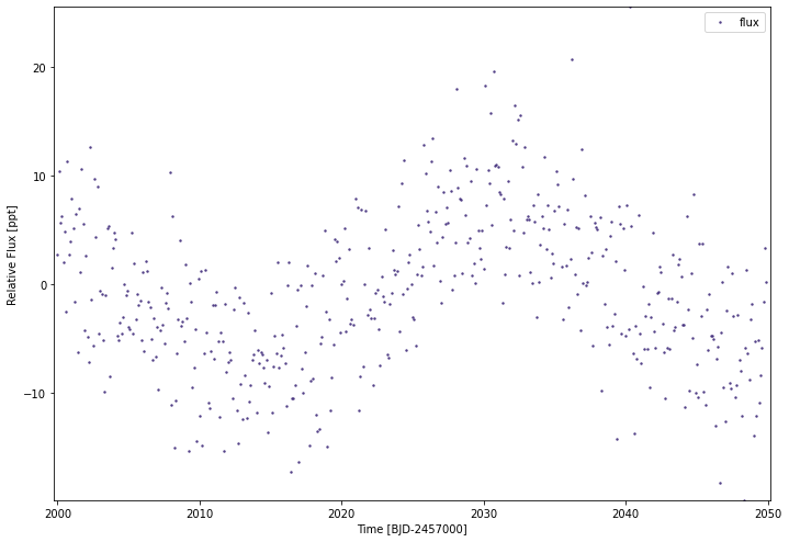
Here is a simple example of loading data:

fakeflux=np.random.normal(7*np.sin(np.linspace(-4,5,500)),5,500)
fakeflux[np.random.choice(500,5)]*=5

simplelc1 = lc.lc()
simplelc1.load_lc(time=np.arange(2000,2050,0.1),
                  fluxes=fakeflux,
                  flux_errs=np.random.normal(0.01,0.0005,500),
                  flx_system='ppt',jd_base=2457000,
                  mission='tess',sect='99',src='test')
simplelc1.plot()

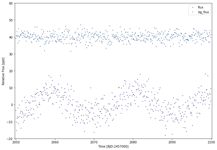
If we have multiple types of flux (for example, ‘raw’ and ‘detrended’ fluxes, background flux, etc) then we can make our input flux and flux_err arguments dictionaries:

fakeflux2=np.random.normal(7*np.sin(np.linspace(5,20,500)),5,500)
fakeflux2[np.random.choice(500,5)]*=5

simplelc2 = lc.lc()
simplelc2.load_lc(time=np.arange(2050,2100,0.1),
                  fluxes={'flux':fakeflux2,'bg_flux':np.random.normal(40,2.5,500)},
                  flux_errs={'flux_err':np.random.normal(0.01,0.0005,500),'bg_flux_err':np.random.normal(2.5,0.01,500)},
                  flx_system='ppt',jd_base=2457000,
                  mission='tess',sect='100',src='test')

#Plotting both of our flux arrays:
simplelc2.plot(timeseries=['flux','bg_flux'],ylim=(-20,60))

One thing to note is the cadence array that is created for these times. This is effectively the unique identifier for the data when stacking lightcurves with the format:

[telescope ID k1/k2/co/te/ch]_[cadence in secs]_[pipeline source]_[Sector/Q/camp]

print(simplelc1.cadence[0])

'ts_8600_test_99'

Masking, binning & flattening

The lightcurve.lc class is built to allow quick masking, binning & flattening of the data.

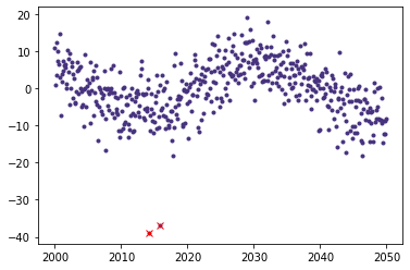
Using lc.make_mask()

This function calls the make_fluxmask function to mask anomalous points.

Some useful arguments when making a mask: * flux_arr_name: Which timeseries of mask * cut_all_anom_lim: The limit in sigma above which we cut all anomalies (default is 5) * end_of_orbit: Whether to mask end-of-orbit flux jumps (often seen in TESS). Default is True * use_flat: Whether to use the flattened flux array to perform masking. Default is False * mask_islands: Whether to mask small “islands” of flux (defined as <0.5d long segments >0.5d from other data). Default is False * input_mask & in_transit: Two already-determined masks which allow inclusion of custom masks and make sure in-transit points are not cut. * extreme_anom_limit: An extreme flux limit above/below which we cut points (default:0.25 meaning flux must be >25% median flux & <400%)

In the case of a multilc (i.e. a lightcurve stacked from multiple sectors/sources), make_cadmask is also called, which masks cadences in the lc.mask_cadences list. This is useful when there are multiple lightcurve sources for the same data (i.e. qlp & pdc), but we only want to consider one as part of the defauly lightcurve as it is higher-quality.

(Note that this is performed by default when accessing a mission lightcurve from lc.multilc)

simplelc1.make_mask()

plt.plot(simplelc1.time,simplelc1.flux,'.')
plt.plot(simplelc1.time[~simplelc1.mask],simplelc1.flux[~simplelc1.mask],'xr')

[<matplotlib.lines.Line2D at 0x7fd97dd45e20>]

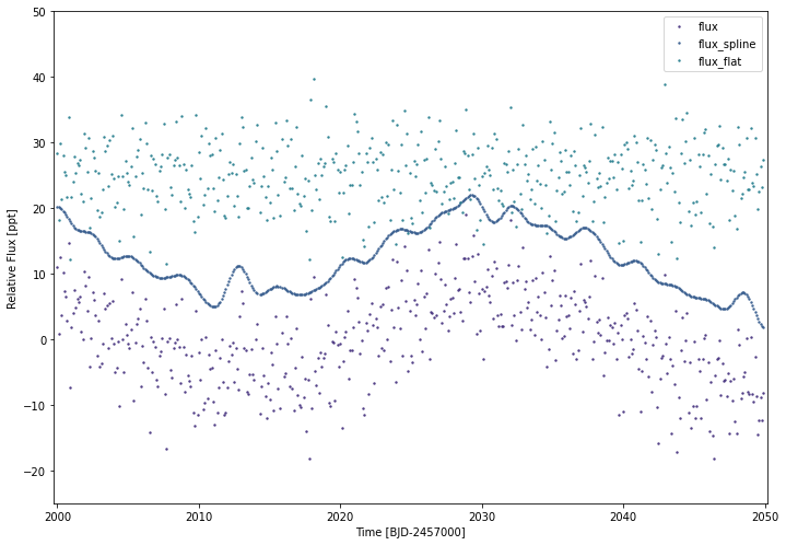
Using lc.flatten()

This is the in-built flattening function. It has two ways of peforming the flattening which can be selected with the flattype argument: - bspline (default): fits smooth splines while iterating away anomalies/transits/etc - polystep: uses out-of-box polynomial fits to smooth data without influencing transit depth

To specify which timeseries to flatten, use the timeseries (default is only the flux array)

To tweak the flattening function, the knot_dist,maxiter,sigmaclip,stepsize, reflect, & polydegree arguments can be used

transit_mask is a key input to the flattten function if transits have been identifed in the timeseries, as this masks the transits from being removed.

lc.flatten() will add a new timeseries to the lc class with the suffix _flat, and in both cases, the best-fit splines are saved to _spline

simplelc1.flatten()
simplelc1.plot(timeseries=['flux','flux_spline','flux_flat'],yoffset=12.5,ylim=(-25,50))

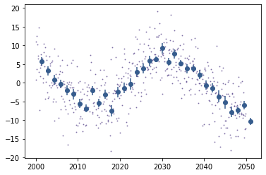
Using lc.bin()

This is the in-built binning function.

Key arguments: * timeseries: As with plot() and flatten(), you can include the timeseries to be binned * binsize, this determines the size of the bines and defaults to 30mins (e.g. 1/48) * use_masked and extramask affect the masks used when binning.

simplelc1.bin(binsize=1.5)

#simplelc1.plot() won't show the bins, as the cadence is too large, so let's go back to a standard plotting:

plt.plot(simplelc1.time[simplelc1.mask],simplelc1.flux[simplelc1.mask],'.',markersize=2,alpha=0.5)
plt.errorbar(simplelc1.bin_time,simplelc1.bin_flux,yerr=simplelc1.bin_flux_err,fmt='o')

<ErrorbarContainer object of 3 artists>

More useful functions

Stacking lc objects

Under the hood of the multilc class is the ability to stack lc objects.

This is done by making a new multilc object (which can be empty) and calling multilc.stack([newlcs]) with a list of lc objects as arguments. For example:

testlc = lc.multilc(123456789,'tess',do_search=False) #we need do_search =False here, as we don't actually want to search for other lightcurves for the star TIC123456789
testlc.stack([simplelc1,simplelc2])
testlc.plot(savepng=False)

Saving

Lightcurves are saved, by default, in the same ID-specific folder that other MonoTools modules access, and which can be modified using the $MONOTOOLSPATH system environment variable but is by default in the MonoTools/data path. So, in this case, it would be in the MonoTools/data/TIC00123456789/ folder.

There are two ways to save the lightcurves found by lc and multilc:

This retainins most metadata, although we delete binned and flattened arrays (which are re-derivable from the other timeseries).

tools.MonoData_savepath

testlc.save()

This does not retain metadata and only stores those timeseries with the same length as the time array (i.e. time, fluxes, flux_errs, cadence, mask, etc):

testlc.save_csv()

#Let's see what got stored:
import pandas as pd
import os
from MonoTools.MonoTools import tools

df=pd.read_csv(os.path.join(tools.MonoData_savepath,"TIC00123456789","TIC00123456789_lc.csv"),index_col=0)
df

	bg_flux	bg_flux_err	cadence	flux	flux_err	flux_mask	flux_spline	mask	time
0	NaN	NaN	ts_8600_test_99	11.022208	0.010108	True	7.669597	True	2459000.0
1	NaN	NaN	ts_8600_test_99	0.809182	0.009523	True	7.631497	True	2459000.1
2	NaN	NaN	ts_8600_test_99	12.440341	0.010081	True	7.514247	True	2459000.2
3	NaN	NaN	ts_8600_test_99	3.618393	0.008787	True	7.329670	True	2459000.3
4	NaN	NaN	ts_8600_test_99	10.173530	0.010226	True	7.089586	True	2459000.4
...	...	...	...	...	...	...	...	...	...
995	42.598741	2.515070	ts_8600_test_100	0.064905	0.009867	True	NaN	True	2459099.5
996	36.871784	2.505943	ts_8600_test_100	6.688908	0.009028	True	NaN	True	2459099.6
997	43.892122	2.487309	ts_8600_test_100	6.159992	0.010139	True	NaN	True	2459099.7
998	39.806309	2.503166	ts_8600_test_100	2.217753	0.010212	True	NaN	True	2459099.8
999	41.508409	2.518718	ts_8600_test_100	9.515834	0.009651	True	NaN	True	2459099.9

1000 rows × 9 columns

Loading

If you have already called multilc with a given id/mission pair, then the data is usually automatically stored in the MonoTools datapath. The next time you call multilc, it will check this path for existing data and load it using multilc.load_pickle(). This can occasionally cause bugs, so often it’s good to check if load=False fixes problems with initialising multilc objects.