Example 1 - Modelling a Duotransit

Let’s walk through how to model a duotransit with MonoTools.

First, some imports:

from MonoTools.MonoTools import fit,tools,starpars,lightcurve

import pandas as pd
import numpy as np
import matplotlib.pyplot as plt
%matplotlib inline

E1 - Loading the lightcurve

Let’s download the target lightcurve using the attached lightcurve module.

use_fast=False means we do not download the 20s cadence data, which slows down the modelling!

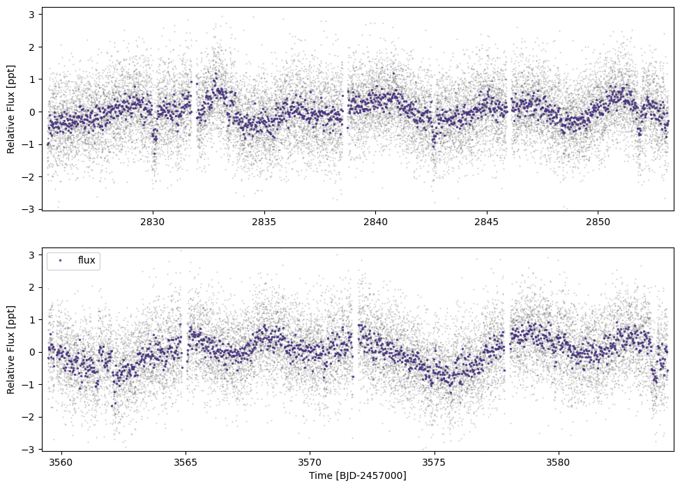
We can then plot the lightcurve using lc.plot() (here we don’t need to save the plot)

tic=431810418
lc=lightcurve.multilc(tic,'tess',save=False,load=False,use_fast=False)
lc.plot(savepng=False,savepdf=False)

Getting all IDs
Accessing online catalogues to match ID to RA/Dec (may be slow) mission= tess
92 91
Sector 92 not (yet) found on MAST | RESPONCE:404
None

ticalc=lightcurve.lc()
sect=83
t=np.hstack([pd.read_csv(f,index_col=0)['time'].values for f in glob.glob("/Users/hugh/Postdoc/Cheops/TICA_lightcurves/TIC"+str(tic)+"_TICA_S*_lc.csv")])
f=np.hstack([1000*(pd.read_csv(f,index_col=0)['flux_ap_1.5'].values/np.nanmedian(pd.read_csv(f,index_col=0)['flux_ap_1.5'])-1) for f in glob.glob("/Users/hugh/Postdoc/Cheops/TICA_lightcurves/TIC"+str(tic)+"_TICA_S*_lc.csv")])
rawf=np.hstack([1000*(pd.read_csv(f,index_col=0)['raw_flux'].values/np.nanmedian(pd.read_csv(f,index_col=0)['raw_flux'])-1) for f in glob.glob("/Users/hugh/Postdoc/Cheops/TICA_lightcurves/TIC"+str(tic)+"_TICA_S*_lc.csv")])
bgf=np.hstack([pd.read_csv(f,index_col=0)['bg_flux'].values for f in glob.glob("/Users/hugh/Postdoc/Cheops/TICA_lightcurves/TIC"+str(tic)+"_TICA_S*_lc.csv")])
ferr=np.hstack([1000*(np.sqrt(pd.read_csv(f,index_col=0)['flux_err'].values)/pd.read_csv(f,index_col=0)['flux_ap_1.5'].values) for f in glob.glob("/Users/hugh/Postdoc/Cheops/TICA_lightcurves/TIC"+str(tic)+"_TICA_S*_lc.csv")])
ticalc.load_lc(time=np.sort(t),
              fluxes={'flux':f[np.argsort(t)],
                      'raw_flux':rawf[np.argsort(t)],
                      'bg_flux':bgf[np.argsort(t)]},
              flux_errs={'flux_err':ferr},
              flx_system='ppt',src='tica',mission='tess',jd_base=2457000,sect=sect)
lc=lightcurve.multilc(tic,'tess',save=False,load=False,extralc=ticalc,priorities=['ts_20_pdc','ts_120_pdc','ts_200_tica'])
lc.plot(savepng=False,savepdf=False)

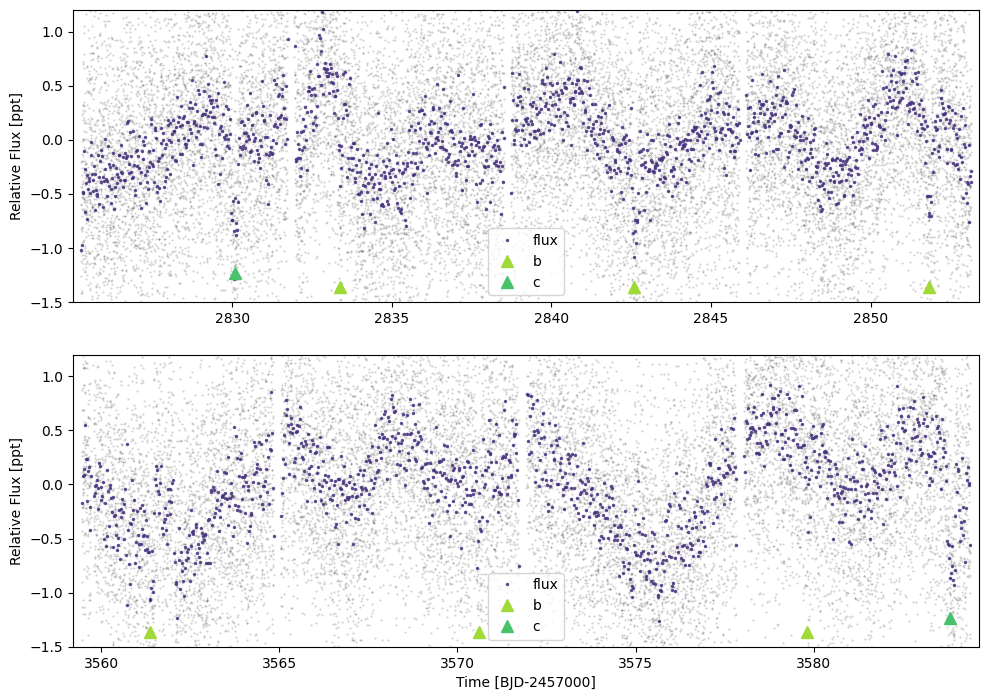
E1 - Plotting the transit positions

By passing a dictionary of dicts to plot_ephem. We also constrain y-axis using ylim:

ephs={'b':{'p':(3570.6-2842.6)/np.round((3570.6-2842.6)/(2851.85-2842.6)),'t0':2842.6,'dur':0.18},
      'c':{'p':(3583.82-2830.1),'t0':3583.82,'dur':0.24}}#Here we just use the transit span as p
lc.plot(plot_ephem=ephs, timeseries=['flux'], ylim=(-1.5,1.2), savepng=False, savepdf=False)

E1 - Initialising the model with a duotransit and multiplanet

The initial fit.monoModel class needs the TIC ID, the mission name, and the lightcurve itself.

Then we can add planets using add_multi and add_duo. These require dictionaries with the ephemeris and depth, as well as (crucially) the planet name.

init_starpars then either takes user-defined stellar parameters (e.g. Rstar=[Rs_med,Rs_neg_err,Rs_pos_err], and same for rhostar, Mstar, logg). In the default case, stellar parameters come from the TIC (v8) catalogue.

We can then initialise the lightcurve and the model

mod=fit.monoModel(tic,'tess',lc=lc)
#mod.add_multi({'tcen':ephs['b']['t0'],'period':ephs['b']['p'],'tdur':ephs['b']['dur'],'depth':0.4e-3},'b')#,update_per=False)
mod.add_multi({'tcen':ephs['b']['t0'],'period':ephs['b']['p'],'tdur':ephs['b']['dur'],'depth':0.55e-3},'b')
mod.add_duo({'tcen':ephs['c']['t0'],'tcen_2':ephs['c']['t0']-ephs['c']['p'],'tdur':ephs['c']['dur'],'depth':0.7e-3},'c')
mod.init_starpars()

{'tcen': 3583.82, 'tcen_2': 2830.1, 'tdur': 0.24, 'depth': 0.0007, 'tcens': array([3583.82, 2830.1 ]), 'span': 753.7200000000003, 'period_int_aliases': array([ 1.,  2.,  3.,  4.,  5.,  6.,  7.,  8.,  9., 10., 11., 12., 13.,
       14., 15., 16., 17., 18., 19., 20., 21., 22., 23., 24., 25., 26.,
       27., 28., 29., 30.])}

E1 - Initialising the lightcurve without a GP

There are two main options - with or without a Gaussian Process.

Without a Gaussian Process (use_GP=False) will use a bspline-fitting method (masking the identified transits). This will be faster, but in cases with relatively high-amplitude noise/stellar activity close in duration to the transit, a GP will be more robust. In this case, we do not need all of the data, so we can cut the out-of-transit data, here to 2.5 transit durations from t0, using cut_distance=2.5.

In the case of use_GP=True, bin_oot=True allows for photometry far-from-transit to be binned in order to speed up computation time. Alternatively, bin_all=True will bin all the data including in-transit points. Alternatively fit_no_flatten=True will not perform any flattening and assume the lightcurve is already flat with out-of-transit flux at ~0.0.

mod.init_lc(use_GP=False, cut_distance=2.5, bin_oot=False)

[2825.25645275 3559.42661067] [2853.1429363  3584.37965094]

E1 - Initialising the duotransit model

There are many options for model fitting:

• constrain_LD=True will constrain the limb darkening coefficients to the theoretical values

• ld_mult=1.5. This is the multiplication factor for the theoretical LD params (to account for systematic errors)

• model_jitter=True will model a log jitter term for each lightcurve (split into cadences)

• model_phot_mean=True will model a mean photometric term for each lightcurve (split into cadences)

• timing_sigma=0.1 allows the adjustment of the priors on the t0s. The default is to assume they are known to ±0.1tdur.

• floattype=np.float64 can be adjusted to e.g. np.float32 to attempt to speed up the model.

• step_initialise=True will optimize the model in steps, starting with the most sensitive transit parameters. This is preferred.

• use_L2=False. If set to True, the model will fit for unincluded “second light” (i.e. contamination)

mod.init_model(constrain_LD=True,ld_mult=1.5,model_jitter=True,model_phot_mean=False,step_initialise=True)

[2825.25645275 3559.42661067] [2853.1429363  3584.37965094]
Initialising ~FAST~ MonoTools model.
initialised planet info
Shape.0
Initialised everything. Optimizing

100.00% [4/4 00:00<00:00 logp = -6,546.2, ||grad|| = 28,660]

100.00% [78/78 00:00<00:00 logp = -6,512.5, ||grad|| = 25,648]

100.00% [45/45 00:00<00:00 logp = -6,511.6, ||grad|| = 5,448.8]

100.00% [39/39 00:00<00:00 logp = -6,511.6, ||grad|| = 13,151]

100.00% [7/7 00:00<00:00 logp = -6,511.6, ||grad|| = 13,151]

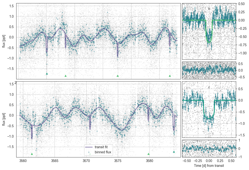
E1 - Plotting the intial duotransit fit

Options here:

• plot_flat=True subtracts the spline fit

• ylim=(-1.5,1.0) sets ylim on full timeseries plot

• xlim=(-0.3,0.3) sets xlim on folded plots

• savepng=False does not save a png (default True)

• savepdf=True saves a pdf (default False)

mod.plot(savepng=False)

initialising transit
Initalising Transit models for plotting with n_samp= 10
phase (5147,) masked_flux 5147 cad_mask 37141 36936 phasebool (37141,) 5183 transmod (5147,) othpls [0. 0. 0. ... 0. 0. 0.] (5147,)
(5147,) (5147,) (5147,) (5147,) (5147,)
phase (1680,) masked_flux 1680 cad_mask 37141 36936 phasebool (37141,) 1680 transmod (1680,) othpls [0. 0. 0. ... 0. 0. 0.] (1680,)
(1680,) (1680,) (1680,) (1680,) (1680,)
0.12964546154463585
0.20641507580074672

E1 - Sampling the duotransit model

The sampling can be modified in the following ways:

• n_draws=1800 is the number of (post-burn-in) samples per chain

• n_chains=6 is the number of chains

• cores=6 is the number of CPU cores to run on.

• sample_method=pm.NUTS allows for the ability to run pymc samplers

mod.sample_model(n_draws=1000,n_chains=6,cores=6)

Multiprocess sampling (6 chains in 6 jobs)
NUTS: [Rs, rhostar, t0_b, per_b, logror_b, b_b, t0_c, logror_c, b_c, tdur_c, q_star_tess, log_jitter_ts_120]

100.00% [9960/9960 11:29<00:00 Sampling 6 chains, 0 divergences]

Sampling 6 chains for 660 tune and 1_000 draw iterations (3_960 + 6_000 draws total) took 690 seconds.
Chain 0 reached the maximum tree depth. Increase `max_treedepth`, increase `target_accept` or reparameterize.
Chain 1 reached the maximum tree depth. Increase `max_treedepth`, increase `target_accept` or reparameterize.
Chain 2 reached the maximum tree depth. Increase `max_treedepth`, increase `target_accept` or reparameterize.
Chain 3 reached the maximum tree depth. Increase `max_treedepth`, increase `target_accept` or reparameterize.
Chain 4 reached the maximum tree depth. Increase `max_treedepth`, increase `target_accept` or reparameterize.
Chain 5 reached the maximum tree depth. Increase `max_treedepth`, increase `target_accept` or reparameterize.
The rhat statistic is larger than 1.01 for some parameters. This indicates problems during sampling. See https://arxiv.org/abs/1903.08008 for details
The effective sample size per chain is smaller than 100 for some parameters.  A higher number is needed for reliable rhat and ess computation. See https://arxiv.org/abs/1903.08008 for details

Saving sampled model parameters to file with shape:  (21, 14)

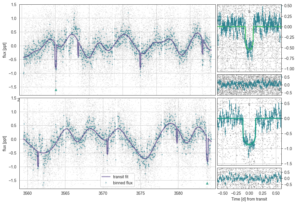
E1 - Plotting the outputs

The models are interpolated to the full input lightcurve and stored in mod.trans_to_plot and mod.gp_to_plot.

overwrite=True re-extracts these transit and spline models from the trace. plot_2sig=True plots both 1 and 2 sigma regions.

mod.plot(overwrite=True, plot_2sig=False,ylim=(-1.8,1.5))

initialising transit
Initalising Transit models for plotting with n_samp= 990
phase (5148,) masked_flux 5148 cad_mask 37141 36936 phasebool (37141,) 5184 transmod (5148,) othpls [0. 0. 0. ... 0. 0. 0.] (5148,)
(5148,) (5148,) (5148,) (5148,) (5148,)
phase (1686,) masked_flux 1686 cad_mask 37141 36936 phasebool (37141,) 1686 transmod (1686,) othpls [0. 0. 0. ... 0. 0. 0.] (1686,)
(1686,) (1686,) (1686,) (1686,) (1686,)
0.13251834087207237
0.17088097275379405

mod.plot_corner()

variables for Corner: ['Rs', 'rhostar', 'logror_b', 'b_b', 'tdur_b', 't0_b', 'logror_c', 'b_c', 'tdur_c', 't0_c']
['Rs', 'rhostar', 'logror_b', 'b_b', 'tdur_b', 't0_b', 'logror_c', 'b_c', 'tdur_c', 't0_c']

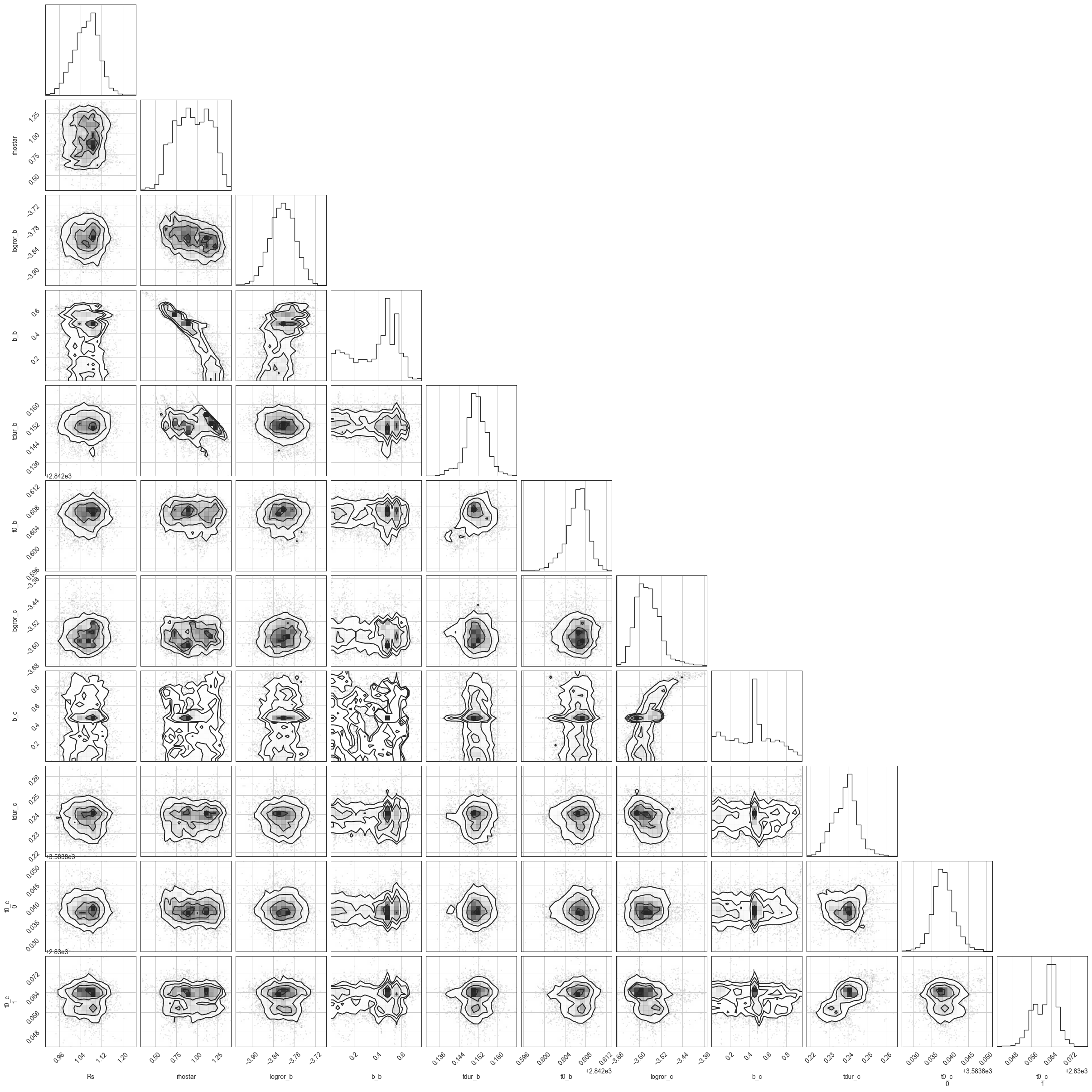
We need to run these models for longer (and potentially prune the b=0.5 outlier here).

E1 - Computing the period probabilities a posteriori

In this new version, we fit the transits in a way ambivalent to the periods, and instead only assess the period probabilities using the trace (and various priors). To do this, you have to call mod.assess_period_from_posterior()

At this point, key choices have to be made about the eccentricity prior by updating ecc_prior='auto'. This is extremely important, as the uncertainty in your derived period distribution depends highly on the eccentricity prior, so choose an option that you believe best matches your planet/planetary system. There are the following options:

• ecc_prior='uniform' - Planets don’t have this distribution in reality. Don’t use this.

• ecc_prior='kipping' - The (close-in) Kipping 2013 prior. Derived from RV planets, and therefore dominated by high-mass planets. Potentially OK in those cases.

• ecc_prior='vaneylen' - Specifically the multi-planet version derived in VanEylen 2018. Measured for compact multi systems in Kepler. The most e=0-biased prior available (therefore, potentially, the best period logprob constraints)

• ecc_prior='bernmodel_sing' - Derived from single planets as produced by Bern model full-system simulations. No observational biases. The Bern Model priors are also all radius-dependent using the initial radius to choose one distribution from [terrestrials, Neptunians or Giants]. The giant case matches kipping well, while the smaller planets are much more low-eccentricity.

• ecc_prior='bernmodel_mult' - Derived from multi systems produced by Bern model. Radius-dependent (rocky, Neptunian & Giants). These, especially for small planets, are well-constrained to e~0 (though less so than vaneylen).

• ecc_prior='bernmodel_both' - Derived from all (observable) planets as produced by Bern model full-system simulations.

• ecc_prior='auto' - The default is the (radius-constrained) bernmodel_both prior for single cases (as we do not know if there could be additional planets), and the bernmodel_mult in multi cases.

mod.assess_period_from_posterior()

multis__bernmodel auto {'kipping': 'kip', 'vaneylen': 'vve', 'flat': 'flat', 'apogee': 'apo', 'bernmodel_both': 'both__bernmodel', 'bernmodel_sing': 'singles__bernmodel', 'bernmodel_mult': 'multis__bernmodel', 'auto': 'multis__bernmodel'} mult ['bern', 'auto']

E1 - Viewing the derived parameters

mod.make_table() creates (and saves) the posterior statistics. Check that ess is at least a thousand, and r_hat is well below 1.05 (ideally below 1.01).

tab=mod.make_table()
tab.to_csv("TOI5968_TIC431810418_best_fit_data.csv")
tab.iloc[:25]

Saving sampled model parameters to file with shape:  (328, 14)

	mean	sd	hdi_3%	hdi_97%	mcse_mean	mcse_sd	ess_bulk	ess_tail	r_hat	5%	-$1\sigma$	median	+$1\sigma$	95%
Rs	1.06189	0.04634	0.97166	1.14453	0.00324	0.00229	221.82731	1076.29584	1.03780	0.98059	1.01383	1.06552	1.10589	1.13321
rhostar	0.94808	0.20533	0.60120	1.29347	0.05671	0.04103	14.06207	84.21169	1.35297	0.62333	0.72072	0.94833	1.17599	1.26266
t0_b	2842.60631	0.00213	2842.60199	2842.61013	0.00014	0.00010	285.45446	239.01105	1.01701	2842.60231	2842.60430	2842.60656	2842.60824	2842.60936
per_b	9.21519	0.00000	9.21518	9.21519	0.00000	0.00000	514.51917	907.03338	1.01120	9.21519	9.21519	9.21519	9.21519	9.21519
logror_b	-3.81360	0.03562	-3.88098	-3.74818	0.00490	0.00349	53.82261	532.60427	1.08189	-3.87322	-3.84942	-3.81321	-3.77804	-3.75564
t0_c[0]	3583.83830	0.00309	3583.83255	3583.84433	0.00016	0.00012	412.95200	405.44537	1.01348	3583.83351	3583.83553	3583.83813	3583.84120	3583.84356
t0_c[1]	2830.06183	0.00471	2830.05276	2830.06977	0.00046	0.00033	114.73809	462.41245	1.04549	2830.05368	2830.05659	2830.06294	2830.06604	2830.06843
logror_c	-3.56762	0.04664	-3.65003	-3.48594	0.00828	0.00593	29.92106	137.17971	1.14933	-3.63306	-3.61136	-3.57202	-3.52643	-3.48636
tdur_c	0.23838	0.00647	0.22511	0.24940	0.00057	0.00040	137.31682	355.47911	1.04165	0.22770	0.23171	0.23882	0.24407	0.24860
log_jitter_ts_120	-1.69956	0.20648	-2.08548	-1.37996	0.01504	0.01126	287.80270	222.07193	1.02313	-2.07737	-1.86880	-1.66404	-1.51849	-1.44411
b_b	0.37342	0.18647	0.03218	0.62246	0.05572	0.04047	11.59547	37.75428	1.46231	0.04395	0.12448	0.43173	0.55124	0.61739
b_c	0.43211	0.24236	0.00245	0.82399	0.03544	0.02522	41.83083	112.67290	1.34701	0.04657	0.13563	0.45777	0.70297	0.84076
q_star_tess[0]	0.25822	0.11404	0.08609	0.44822	0.03049	0.02203	15.62891	45.80557	1.29616	0.09516	0.10801	0.26694	0.37700	0.43494
q_star_tess[1]	0.31133	0.08084	0.15013	0.45902	0.00759	0.00538	98.04540	268.07579	1.06967	0.17087	0.22746	0.31646	0.38585	0.43959
ror_b	0.02208	0.00078	0.02063	0.02356	0.00011	0.00008	53.82261	532.60427	1.08189	0.02079	0.02129	0.02208	0.02287	0.02339
rpl_b	2.56080	0.14648	2.29119	2.82569	0.01248	0.00885	141.23675	839.90987	1.06038	2.32404	2.41444	2.55604	2.71575	2.79701
ror_c	0.02825	0.00135	0.02598	0.03062	0.00024	0.00017	29.92106	137.17971	1.14933	0.02644	0.02702	0.02810	0.02941	0.03061
rpl_c	3.27645	0.21393	2.88626	3.67140	0.03327	0.02369	40.57589	490.06167	1.10783	2.95276	3.07038	3.25759	3.49000	3.63663
u_star_tess[0]	0.30612	0.10903	0.13735	0.52392	0.02122	0.01517	27.14605	177.41133	1.17004	0.15056	0.19896	0.29476	0.42089	0.49796
u_star_tess[1]	0.18736	0.09888	0.01520	0.37797	0.01780	0.01271	31.48817	279.15544	1.14207	0.04883	0.09800	0.16650	0.28974	0.36947
tdur_b	0.15111	0.00436	0.14202	0.15958	0.00043	0.00031	120.46246	108.80107	1.04323	0.14332	0.14744	0.15112	0.15523	0.15803
pcirc_c	0.00000	0.00000	0.00000	0.00000	0.00000	0.00000	45.60024	129.94365	1.33323	0.00000	0.00000	0.00000	0.00000	0.00000
per_c[0]	753.77647	0.00575	753.76722	753.78792	0.00053	0.00038	114.17134	447.75035	1.04615	753.76834	753.77111	753.77585	753.78231	753.78672
per_c[1]	376.88824	0.00287	376.88361	376.89396	0.00027	0.00019	114.17134	447.75035	1.04615	376.88417	376.88556	376.88793	376.89115	376.89336
per_c[2]	251.25882	0.00192	251.25574	251.26264	0.00018	0.00013	114.17134	447.75035	1.04615	251.25611	251.25704	251.25862	251.26077	251.26224

E1 - Plotting the orbital period posterior probability distribution

This is, in many ways, the key figure. What is the most likely orbital period?

Options: ymin=-4, pmin=23, pmax=300, etc.

mod.plot_periods(ymin=-4)

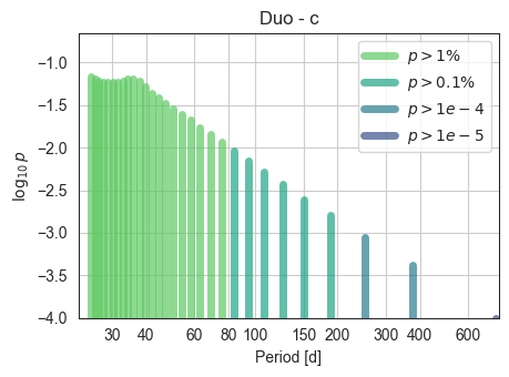
The general decreasing trend is due to the various priors (geometric, etc) which prefer short periods. The “bump” here is likely due to the circular/low eccentricity regime peaking around this value. A more constraining eccentricity prior may change the result…

E1 - Saving the duotranist model

mod.save_model_to_file()

E1 - Predicting upcoming transits for all aliases

Using mod.predict_future_transits()

• We can specify a time range using time_start and time_end via astropy.time.Time objects (time_end=Time("2026-01-01T00:00:00.0",format='isot')), or use time_dur=500 to ask for a prediction 500 days into the future.

• We can check which transits are TESS observed using check_TESS=True (default)

• We can use compute_solsys_dist=True to compute sun and moon distances (CHEOPS observations are possible when sun_dist>117 and moon_dist>15).

trans=mod.predict_future_transits(time_dur=500)
trans.to_csv("TOI5968_TIC431810418_trans_table.csv")

time range 2025-06-05T15:50:38.491 -> 2026-10-18T15:50:38.492

trans

	transit_mid_date	transit_mid_med	transit_dur_med	transit_dur_-1sig	transit_dur_+1sig	transit_start_+2sig	transit_start_+1sig	transit_start_med	transit_start_-1sig	transit_start_-2sig	...	planet_name	alias_n	alias_p	aliases_ns	aliases_ps	total_prob	num_aliases	in_TESS	sun_separation	moon_separation
0	2025-06-11T08:19:46.470	3837.847066	0.151122	0.147437	0.155233	3837.780293	3837.775057	3837.771504	3837.767152	3837.761926	...	multi_b	0	9.21519	0	9.2152	1.0	1.0	False	78.389208	104.101889
1	2025-06-20T13:29:38.506	3847.062251	0.151122	0.147437	0.155233	3846.995484	3846.990248	3846.986690	3846.982342	3846.977116	...	multi_b	0	9.21519	0	9.2152	1.0	1.0	False	85.759439	34.597295
2	2025-06-29T18:39:30.858	3856.277440	0.151122	0.147437	0.155233	3856.210674	3856.205440	3856.201879	3856.197533	3856.192305	...	multi_b	0	9.21519	0	9.2152	1.0	1.0	False	93.154198	135.076334
3	2025-07-08T23:49:23.402	3865.492632	0.151122	0.147437	0.155233	3865.425865	3865.420632	3865.417071	3865.412723	3865.407495	...	multi_b	0	9.21519	0	9.2152	1.0	1.0	False	100.520485	100.490479
4	2025-07-18T04:59:15.844	3874.707822	0.151122	0.147437	0.155233	3874.641056	3874.635824	3874.632261	3874.627914	3874.622685	...	multi_b	0	9.21519	0	9.2152	1.0	1.0	False	107.811175	36.950328
5	2025-07-27T10:09:08.164	3883.923011	0.151122	0.147437	0.155233	3883.856244	3883.851016	3883.847450	3883.843103	3883.837874	...	multi_b	0	9.21519	0	9.2152	1.0	1.0	False	114.972771	137.466355
6	2025-08-05T15:19:00.702	3893.138203	0.151122	0.147437	0.155233	3893.071435	3893.066207	3893.062641	3893.058292	3893.053062	...	multi_b	0	9.21519	0	9.2152	1.0	1.0	False	121.918730	97.328477
7	2025-08-14T20:28:53.184	3902.353393	0.151122	0.147437	0.155233	3902.286626	3902.281398	3902.277832	3902.273482	3902.268249	...	multi_b	0	9.21519	0	9.2152	1.0	1.0	False	128.531425	40.122646
8	2025-08-24T01:38:45.491	3911.568582	0.151122	0.147437	0.155233	3911.501817	3911.496588	3911.493021	3911.488671	3911.483437	...	multi_b	0	9.21519	0	9.2152	1.0	1.0	False	134.641085	139.822349
9	2025-09-02T06:48:37.888	3920.783772	0.151122	0.147437	0.155233	3920.717004	3920.711777	3920.708211	3920.703860	3920.698624	...	multi_b	0	9.21519	0	9.2152	1.0	1.0	False	139.976969	94.383946
10	2025-09-11T11:58:30.314	3929.998962	0.151122	0.147437	0.155233	3929.932193	3929.926968	3929.923401	3929.919051	3929.913812	...	multi_b	0	9.21519	0	9.2152	1.0	1.0	False	144.153345	43.525182
11	2025-09-20T17:08:22.687	3939.214151	0.151122	0.147437	0.155233	3939.147384	3939.142158	3939.138590	3939.134243	3939.128999	...	multi_b	0	9.21519	0	9.2152	1.0	1.0	False	146.697717	142.279675
12	2025-09-29T22:18:15.108	3948.429342	0.151122	0.147437	0.155233	3948.362575	3948.357348	3948.353780	3948.349433	3948.344186	...	multi_b	0	9.21519	0	9.2152	1.0	1.0	False	147.187220	91.238089
13	2025-10-09T03:28:07.458	3957.644531	0.151122	0.147437	0.155233	3957.577766	3957.572539	3957.568970	3957.564624	3957.559374	...	multi_b	0	9.21519	0	9.2152	1.0	1.0	False	145.501102	46.468435
14	2025-10-18T08:37:59.837	3966.859720	0.151122	0.147437	0.155233	3966.792957	3966.787729	3966.784159	3966.779815	3966.774561	...	multi_b	0	9.21519	0	9.2152	1.0	1.0	False	141.900768	144.723997
15	2025-10-27T13:47:52.173	3976.074909	0.151122	0.147437	0.155233	3976.008148	3976.002920	3975.999348	3975.995005	3975.989748	...	multi_b	0	9.21519	0	9.2152	1.0	1.0	False	136.841509	87.560533
16	2025-11-05T18:57:44.634	3985.290100	0.151122	0.147437	0.155233	3985.223339	3985.218112	3985.214539	3985.210194	3985.204936	...	multi_b	0	9.21519	0	9.2152	1.0	1.0	False	130.763292	48.660160
17	2025-11-15T00:07:37.039	3994.505290	0.151122	0.147437	0.155233	3994.438530	3994.433303	3994.429729	3994.425379	3994.420124	...	multi_b	0	9.21519	0	9.2152	1.0	1.0	False	123.992418	146.854374
18	2025-11-24T05:17:29.423	4003.720479	0.151122	0.147437	0.155233	4003.653719	4003.648495	4003.644918	4003.640570	4003.635313	...	multi_b	0	9.21519	0	9.2152	1.0	1.0	False	116.752230	83.368881
19	2025-12-03T10:27:21.702	4012.935668	0.151122	0.147437	0.155233	4012.868909	4012.863685	4012.860107	4012.855758	4012.850502	...	multi_b	0	9.21519	0	9.2152	1.0	1.0	False	109.204775	50.551928
20	2025-12-12T15:37:14.097	4022.150858	0.151122	0.147437	0.155233	4022.084098	4022.078876	4022.075296	4022.070946	4022.065691	...	multi_b	0	9.21519	0	9.2152	1.0	1.0	False	101.461238	148.399419
21	2025-12-21T20:47:06.625	4031.366049	0.151122	0.147437	0.155233	4031.299290	4031.294066	4031.290488	4031.286134	4031.280879	...	multi_b	0	9.21519	0	9.2152	1.0	1.0	False	93.601817	79.058327
22	2025-12-31T01:56:59.091	4040.581239	0.151122	0.147437	0.155233	4040.514482	4040.509258	4040.505678	4040.501321	4040.496068	...	multi_b	0	9.21519	0	9.2152	1.0	1.0	False	85.705442	53.063147
23	2026-01-09T07:06:51.705	4049.796432	0.151122	0.147437	0.155233	4049.729675	4049.724448	4049.720871	4049.716509	4049.711256	...	multi_b	0	9.21519	0	9.2152	1.0	1.0	False	77.843998	149.295272
24	2026-01-18T12:16:44.218	4059.011623	0.151122	0.147437	0.155233	4058.944868	4058.939639	4058.936062	4058.931699	4058.926445	...	multi_b	0	9.21519	0	9.2152	1.0	1.0	False	70.085340	75.140034
25	2026-01-27T17:26:36.638	4068.226813	0.151122	0.147437	0.155233	4068.160059	4068.154829	4068.151252	4068.146889	4068.141633	...	multi_b	0	9.21519	0	9.2152	1.0	1.0	False	62.523603	56.784796
26	2026-02-05T22:36:28.892	4077.442001	0.151122	0.147437	0.155233	4077.375249	4077.370020	4077.366440	4077.362079	4077.356821	...	multi_b	0	9.21519	0	9.2152	1.0	1.0	False	55.282020	149.644375
27	2026-02-15T03:46:21.284	4086.657191	0.151122	0.147437	0.155233	4086.590437	4086.585209	4086.581630	4086.577269	4086.572010	...	multi_b	0	9.21519	0	9.2152	1.0	1.0	False	48.521447	71.851359
28	2026-02-24T08:56:13.858	4095.872383	0.151122	0.147437	0.155233	4095.805630	4095.800397	4095.796821	4095.792458	4095.787198	...	multi_b	0	9.21519	0	9.2152	1.0	1.0	False	42.488808	61.482701
29	2026-03-05T14:06:06.354	4105.087574	0.151122	0.147437	0.155233	4105.020820	4105.015587	4105.012012	4105.007650	4105.002386	...	multi_b	0	9.21519	0	9.2152	1.0	1.0	False	37.542999	149.539845
30	2026-03-14T19:15:58.860	4114.302765	0.151122	0.147437	0.155233	4114.236008	4114.230775	4114.227203	4114.222837	4114.217575	...	multi_b	0	9.21519	0	9.2152	1.0	1.0	False	34.141145	68.964285
31	2026-03-24T00:25:51.370	4123.517956	0.151122	0.147437	0.155233	4123.451198	4123.445966	4123.442394	4123.438024	4123.432763	...	multi_b	0	9.21519	0	9.2152	1.0	1.0	False	32.745840	66.343913
32	2026-04-02T05:35:43.694	4132.733145	0.151122	0.147437	0.155233	4132.666384	4132.661157	4132.657583	4132.653216	4132.647952	...	multi_b	0	9.21519	0	9.2152	1.0	1.0	False	33.579042	148.949546
33	2026-04-11T10:45:35.966	4141.948333	0.151122	0.147437	0.155233	4141.881570	4141.876347	4141.872772	4141.868404	4141.863140	...	multi_b	0	9.21519	0	9.2152	1.0	1.0	False	36.452822	65.990259
34	2026-04-20T15:55:28.445	4151.163524	0.151122	0.147437	0.155233	4151.096757	4151.091539	4151.087962	4151.083592	4151.078328	...	multi_b	0	9.21519	0	9.2152	1.0	1.0	False	40.908742	70.567271
35	2026-04-29T21:05:20.778	4160.378713	0.151122	0.147437	0.155233	4160.311944	4160.306729	4160.303152	4160.298783	4160.293517	...	multi_b	0	9.21519	0	9.2152	1.0	1.0	False	46.459726	147.755239
36	2026-05-09T02:15:13.220	4169.593903	0.151122	0.147437	0.155233	4169.527135	4169.521917	4169.518342	4169.513973	4169.508707	...	multi_b	0	9.21519	0	9.2152	1.0	1.0	False	52.730616	62.564579
37	2026-05-18T07:25:05.605	4178.809093	0.151122	0.147437	0.155233	4178.742326	4178.737105	4178.733531	4178.729161	4178.723896	...	multi_b	0	9.21519	0	9.2152	1.0	1.0	False	59.471033	73.833005
38	2026-05-27T12:34:57.914	4188.024281	0.151122	0.147437	0.155233	4187.957518	4187.952295	4187.948720	4187.944353	4187.939085	...	multi_b	0	9.21519	0	9.2152	1.0	1.0	False	66.508624	145.939190
39	2026-06-05T17:44:50.358	4197.239472	0.151122	0.147437	0.155233	4197.172708	4197.167486	4197.163911	4197.159543	4197.154275	...	multi_b	0	9.21519	0	9.2152	1.0	1.0	False	73.729766	58.658971
40	2026-06-14T22:54:42.695	4206.454661	0.151122	0.147437	0.155233	4206.387898	4206.382675	4206.379100	4206.374732	4206.369464	...	multi_b	0	9.21519	0	9.2152	1.0	1.0	False	81.063686	76.466514
41	2026-06-24T04:04:35.128	4215.669851	0.151122	0.147437	0.155233	4215.603090	4215.597863	4215.594290	4215.589921	4215.584653	...	multi_b	0	9.21519	0	9.2152	1.0	1.0	False	88.449773	143.692978
42	2026-07-03T09:14:27.499	4224.885040	0.151122	0.147437	0.155233	4224.818285	4224.813054	4224.809479	4224.805110	4224.799842	...	multi_b	0	9.21519	0	9.2152	1.0	1.0	False	95.835653	54.544327
43	2026-07-12T14:24:19.704	4234.100228	0.151122	0.147437	0.155233	4234.033479	4234.028247	4234.024667	4234.020299	4234.015030	...	multi_b	0	9.21519	0	9.2152	1.0	1.0	False	103.181785	79.205636
44	2026-07-21T19:34:12.109	4243.315418	0.151122	0.147437	0.155233	4243.248670	4243.243437	4243.239857	4243.235488	4243.230219	...	multi_b	0	9.21519	0	9.2152	1.0	1.0	False	110.436012	141.298358
45	2026-07-31T00:44:04.425	4252.530607	0.151122	0.147437	0.155233	4252.463861	4252.458627	4252.455046	4252.450677	4252.445407	...	multi_b	0	9.21519	0	9.2152	1.0	1.0	False	117.526594	50.624329
46	2026-08-09T05:53:56.740	4261.745796	0.151122	0.147437	0.155233	4261.679052	4261.673818	4261.670234	4261.665866	4261.660596	...	multi_b	0	9.21519	0	9.2152	1.0	1.0	False	124.367474	82.728558
47	2026-08-18T11:03:49.252	4270.960987	0.151122	0.147437	0.155233	4270.894243	4270.889009	4270.885426	4270.881056	4270.875785	...	multi_b	0	9.21519	0	9.2152	1.0	1.0	False	130.825027	138.923806
48	2026-08-27T16:13:41.621	4280.176176	0.151122	0.147437	0.155233	4280.109434	4280.104201	4280.100615	4280.096245	4280.090974	...	multi_b	0	9.21519	0	9.2152	1.0	1.0	False	136.687632	47.234343
49	2026-09-05T21:23:34.272	4289.391369	0.151122	0.147437	0.155233	4289.324624	4289.319390	4289.315808	4289.311433	4289.306163	...	multi_b	0	9.21519	0	9.2152	1.0	1.0	False	141.651812	87.266055
50	2026-09-15T02:33:26.784	4298.606560	0.151122	0.147437	0.155233	4298.539814	4298.534580	4298.530999	4298.526622	4298.521350	...	multi_b	0	9.21519	0	9.2152	1.0	1.0	False	145.294235	136.520918
51	2026-09-24T07:43:18.986	4307.821748	0.151122	0.147437	0.155233	4307.755004	4307.749772	4307.746186	4307.741811	4307.736538	...	multi_b	0	9.21519	0	9.2152	1.0	1.0	False	147.128490	44.460905
52	2026-10-03T12:53:11.405	4317.036938	0.151122	0.147437	0.155233	4316.970196	4316.964962	4316.961376	4316.957000	4316.951727	...	multi_b	0	9.21519	0	9.2152	1.0	1.0	False	146.819383	92.487169
53	2026-10-12T18:03:03.884	4326.252128	0.151122	0.147437	0.155233	4326.185388	4326.180150	4326.176567	4326.172188	4326.166920	...	multi_b	0	9.21519	0	9.2152	1.0	1.0	False	144.390519	133.878554

54 rows × 30 columns

# Pre-initialisation step (for me) to run before the rest of the notebook
# The followg may need to be MonoTools.MonoTools if you are outside the MonoTools folder when importing:
import os
os.environ['MONOTOOLSPATH']='/Users/hugh/Postdoc/Cheops/Duotransits'
import pytensor
pytensor.config.gcc__cxxflags = '-fbracket-depth=512'
%load_ext autoreload
%autoreload 2