Example 4 - an amiguous transit signal with TTVs & GPs
We will refit the model from example 3 with 5 non-consecutive transits, but include GPs and TTVs.
[16]:
import numpy as np
import pandas as pd
import os
import arviz as az
import matplotlib.pyplot as plt
%matplotlib inline
from MonoTools.MonoTools import fit, tools, lightcurve
The autoreload extension is already loaded. To reload it, use:
  %reload_ext autoreload
E4 - Downloading the TESS lightcurve
As for the previous “simple” notebook, we need to do some cleaning due to noisy parts of the most recent TESS sector
[4]:
tic=103095888
lc=lightcurve.multilc(tic,'tess',save=False)
lc.mask[abs(lc.time-3654.5)<4.8]=False
lc.mask[abs(lc.time-3638.5)<1.75]=False
lc.remove_binned_arrs()
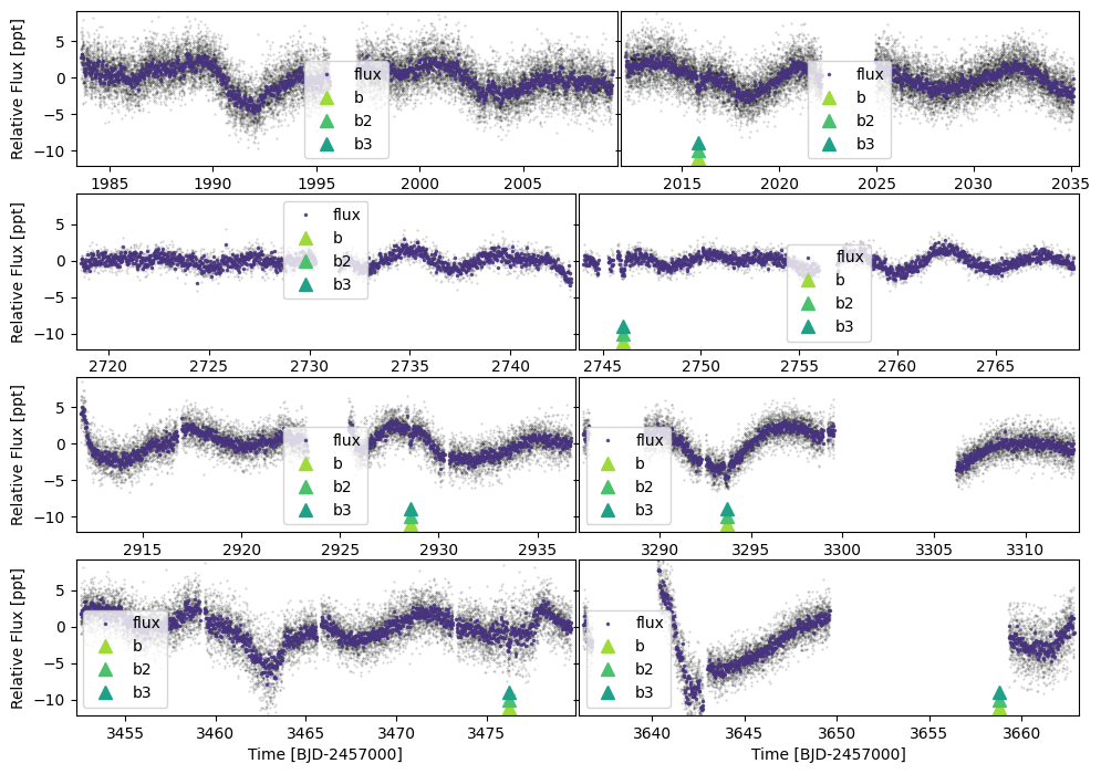
lc.plot(timeseries=['flux'],plot_ephem={'b':{'p':(2746.02021-2015.81701)/4,'t0':2746.02021},
'b2':{'p':(2746.02021-2015.81701)/8,'t0':2746.02021},
'b3':{'p':(2746.02021-2015.81701)/20,'t0':2746.02021}},savepng=False)
Getting all IDs
Accessing online catalogues to match ID to RA/Dec (may be slow) mission= tess
92 91
Sector 92 not (yet) found on MAST | RESPONCE:404
['/Users/hugh/Postdoc/MonoTools_working/TIC00103095888/orbit-45_qlplc.h5', '/Users/hugh/Postdoc/MonoTools_working/TIC00103095888/orbit-46_qlplc.h5']
['/Users/hugh/Postdoc/MonoTools_working/TIC00103095888/orbit-165_qlplc.h5', '/Users/hugh/Postdoc/MonoTools_working/TIC00103095888/orbit-166_qlplc.h5']
['/Users/hugh/Postdoc/MonoTools_working/TIC00103095888/orbit-179_qlplc.h5', '/Users/hugh/Postdoc/MonoTools_working/TIC00103095888/orbit-180_qlplc.h5']
None
E4 - Intialising the ambiguous transit model
[5]:
mod = fit.monoModel(tic, 'tess', lc=lc)
mod.init_starpars()
mod.add_ambiguous({'tcens':[2015.81701,
                            np.random.normal(2746.02021,0.015),
                            np.random.normal(2928.57101,0.015),
                            np.random.normal(3293.67261,0.015),
                            3476.22341],
                   'tdur':10/48,'depth':1.8e-3},'b')
{'tcens': array([2015.81701   , 2746.05279447, 2928.55541517, 3293.66671314,
       3476.22341   ]), 'tdur': 0.20833333333333334, 'depth': 0.0018, 'span': 1460.4064, 'maxperiod_pair': 1, 'maxperiod': 182.5508, 'p_ratios': array([[[ 8., 16., 24., 32., 40., 48., 56., 64., 72., 80., 88., 96.],
        [ 4.,  8., 12., 16., 20., 24., 28., 32., 36., 40., 44., 48.]],

       [[ 8., 16., 24., 32., 40., 48., 56., 64., 72., 80., 88., 96.],
        [ 5., 10., 15., 20., 25., 30., 35., 40., 45., 50., 55., 60.]],

       [[ 8., 16., 24., 32., 40., 48., 56., 64., 72., 80., 88., 96.],
        [ 7., 14., 21., 28., 35., 42., 49., 56., 63., 70., 77., 84.]],

       [[ 8., 16., 24., 32., 40., 48., 56., 64., 72., 80., 88., 96.],
        [ 8., 16., 24., 32., 40., 48., 56., 64., 72., 80., 88., 96.]]]), 'period': 182.5508, 'period_err': 0.034708333333333334, 'period_int_aliases': array([ 8., 16., 24., 32., 40.])}
E4 - Initialising the lightcurve with GPs
Here we can set use_GP=True which means a celerite simple harmonic osscilator Gaussian Process will be co-modelled alongside the transit models.
Using bin_oot=True and cut_distance=1.25 means that photometry more than 1.25 transit durations away from the transit centres will be binned (to 30mins).
By default, train_GP=True, which means that out-of-transit data is inially fit with a GP. This will help assess the lightcurve GP hyperparameters in order to set relatively constraining priors. These priors can be simple Gaussians, or more complex interpolated functions using gp_prior_interp=True (though covariances are ignored).
Another possibility is to set a periodic_kernel (None by default). Passing a dictionary featuringperiod, logamp, logamp_err and periodic_Q here will initialise a periodic (i.e. stellar rotation) kernel on top of the SHO kernel.
[6]:
mod.init_lc(use_GP=True, bin_oot=True, cut_distance=1.25, model_ambig_ttv=True,train_GP=True)
[False False False ... False False False]
{'time': (2499,), 'flux': (2499,), 'flux_err': (2499,), 'near_trans': (2499,), 'in_trans': (2499,)}
[False False False ... False False False]
{'time': (5191,), 'flux': (5191,), 'flux_err': (5191,), 'near_trans': (5191,), 'in_trans': (5191,)}
[False False False ... False False False]
{'time': (2288,), 'flux': (2288,), 'flux_err': (2288,), 'near_trans': (2288,), 'in_trans': (2288,)}
E4 - Initialising the model
Modelling TTVs for trio/quad/etcs
By stating model_ambig_ttv=True we are instead going to model individual transit times and then derive a global period from those. Otherwise, the model fits two transit times (the first and last) and derives intermediate transit times assuming a linear ephemeris and the pre-determined period ratio with respect to the total span
[140]:
mod.init_model(use_GP=True, bin_oot=True, cut_distance=1.25, model_ambig_ttv=True)
Initialising ~FAST~ MonoTools model.
initialised planet info
Shape.0
Initialised everything. Optimizing
[137]:
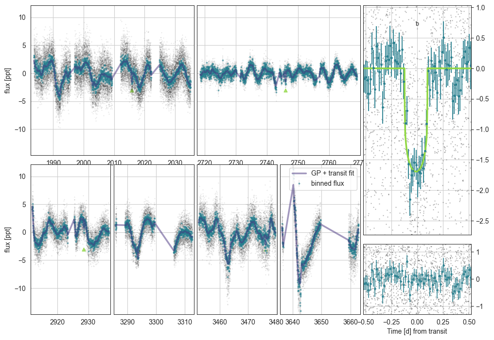
mod.plot()
initialising transit
Initalising Transit models for plotting with n_samp= 10
ts_120 successfully interpolated GP means
ts_200 successfully interpolated GP means
ts_600 successfully interpolated GP means
0.2587202715131996
E4 - Sampling the model
This is slower than the simple case.
[142]:
mod.sample_model(overwrite=True, cores=6, n_draws=800)
Multiprocess sampling (6 chains in 6 jobs)
NUTS: [Rs, rhostar, t0_b, logror_b, b_b, tdur_b, q_star_tess, log_jitter_ts_120, phot_mean_ts_120, log_jitter_ts_200, phot_mean_ts_200, log_jitter_ts_600, phot_mean_ts_600, phot_w0, phot_sigma]
Sampling 6 chains for 528 tune and 800 draw iterations (3_168 + 4_800 draws total) took 5079 seconds.
Chain 0 reached the maximum tree depth. Increase `max_treedepth`, increase `target_accept` or reparameterize.
Chain 1 reached the maximum tree depth. Increase `max_treedepth`, increase `target_accept` or reparameterize.
Chain 2 reached the maximum tree depth. Increase `max_treedepth`, increase `target_accept` or reparameterize.
Chain 3 reached the maximum tree depth. Increase `max_treedepth`, increase `target_accept` or reparameterize.
Chain 4 reached the maximum tree depth. Increase `max_treedepth`, increase `target_accept` or reparameterize.
Chain 5 reached the maximum tree depth. Increase `max_treedepth`, increase `target_accept` or reparameterize.
The rhat statistic is larger than 1.01 for some parameters. This indicates problems during sampling. See https://arxiv.org/abs/1903.08008 for details
The effective sample size per chain is smaller than 100 for some parameters.  A higher number is needed for reliable rhat and ess computation. See https://arxiv.org/abs/1903.08008 for details
Saving sampled model parameters to file with shape: (9257, 14)
[149]:
_=az.plot_trace(mod.trace['posterior'], var_names=['b_b','logror_b','tdur_b','q_star_tess','log_jitter_ts_120','log_jitter_ts_200'])
#warmup_posterior

We need way more samples here. But this is just a demo.
[150]:
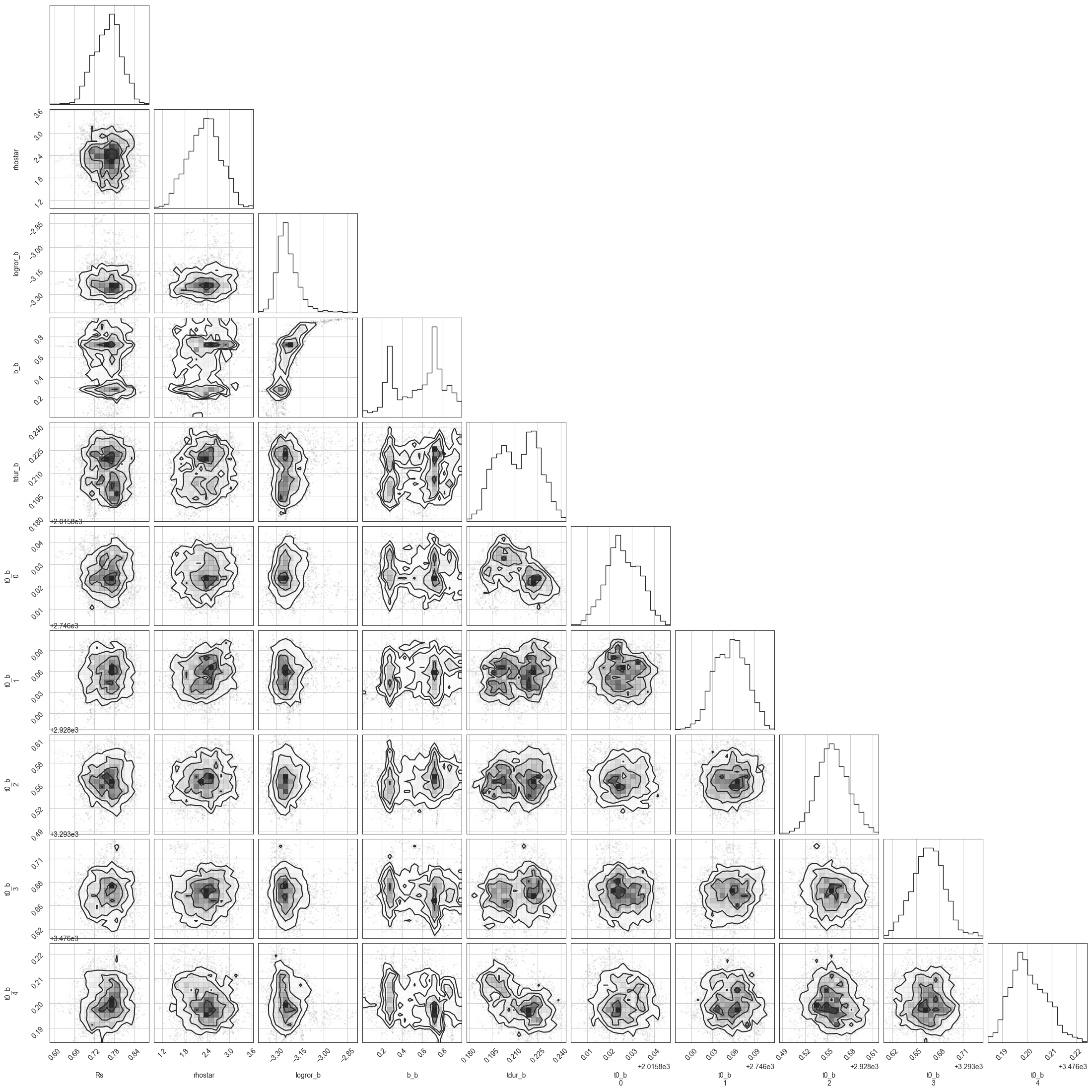
mod.plot_corner()
variables for Corner: ['Rs', 'rhostar', 'logror_b', 'b_b', 'tdur_b', 't0_b']
['Rs', 'rhostar', 'logror_b', 'b_b', 'tdur_b', 't0_b']
E4 - Plotting the best-fit
[153]:
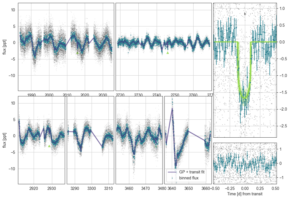
mod.plot()
initialising transit
Initalising Transit models for plotting with n_samp= 990
0.29085769063688505
E4 - Computing the posterior period probabilities
[205]:
mod.assess_period_from_posterior()
both__bernmodel auto {'kipping': 'kip', 'vaneylen': 'vve', 'flat': 'flat', 'apogee': 'apo', 'bernmodel_both': 'both__bernmodel', 'bernmodel_sing': 'singles__bernmodel', 'bernmodel_mult': 'multis__bernmodel', 'auto': 'both__bernmodel'} both ['bern', 'auto']
E4 - Final outputs
Plotting period aliases:
[207]:
mod.plot_periods(ymin=-2.5)

Posterior table
[215]:
mod.make_table()
Saving sampled model parameters to file with shape: (9314, 14)
[215]:
| mean | sd | hdi_3% | hdi_97% | mcse_mean | mcse_sd | ess_bulk | ess_tail | r_hat | 5% | -$1\sigma$ | median | +$1\sigma$ | 95% | |
|---|---|---|---|---|---|---|---|---|---|---|---|---|---|---|
| Rs | 0.75903 | 0.04050 | 0.68584 | 0.83318 | 0.00316 | 0.00224 | 171.01372 | 579.84759 | 1.03478 | 0.69107 | 0.71511 | 0.76219 | 0.79868 | 0.82463 |
| rhostar | 2.33074 | 0.43892 | 1.52493 | 3.12482 | 0.04886 | 0.03497 | 81.43689 | 167.81385 | 1.07551 | 1.58759 | 1.86375 | 2.34572 | 2.77562 | 3.04480 |
| t0_b[0] | 2015.82597 | 0.00735 | 2015.81237 | 2015.83956 | 0.00125 | 0.00089 | 36.28396 | 247.07322 | 1.14869 | 2015.81376 | 2015.81873 | 2015.82557 | 2015.83394 | 2015.83783 |
| t0_b[1] | 2746.05598 | 0.02272 | 2746.01700 | 2746.09961 | 0.00372 | 0.00265 | 37.89330 | 95.03845 | 1.11385 | 2746.01937 | 2746.03170 | 2746.05707 | 2746.07950 | 2746.09370 |
| t0_b[2] | 2928.55699 | 0.02090 | 2928.51941 | 2928.59772 | 0.00187 | 0.00133 | 125.70602 | 296.18575 | 1.02444 | 2928.52335 | 2928.53611 | 2928.55628 | 2928.57823 | 2928.59301 |
| ... | ... | ... | ... | ... | ... | ... | ... | ... | ... | ... | ... | ... | ... | ... |
| ecc_marg_av_b | 0.30971 | 0.16610 | 0.07270 | 0.65055 | 0.04126 | 0.02971 | 15.81982 | 34.17540 | 1.32507 | 0.12329 | 0.14933 | 0.24883 | 0.42684 | 0.67428 |
| ecc_marg_sd_b | 0.01365 | 0.00895 | 0.00419 | 0.03019 | 0.00196 | 0.00141 | 18.67613 | 82.13914 | 1.22990 | 0.00507 | 0.00702 | 0.01110 | 0.02029 | 0.03148 |
| vel_marg_b | 0.83900 | 0.17135 | 0.45918 | 1.10454 | 0.04475 | 0.03336 | 14.32403 | 34.47314 | 1.37040 | 0.48740 | 0.71350 | 0.88434 | 1.00367 | 1.06360 |
| per_marg_av_b | 56.07264 | 7.93798 | 40.63602 | 68.56733 | 2.07976 | 1.50111 | 13.54872 | 78.48915 | 1.39225 | 41.87952 | 46.59363 | 56.45058 | 62.43775 | 68.64177 |
| per_marg_sd_b | 1056.02463 | 884.80687 | 73.11456 | 2713.21873 | 251.40179 | 182.13025 | 12.32250 | 71.14970 | 1.46362 | 149.00842 | 188.08279 | 852.28493 | 1894.09121 | 2830.57632 |
9314 rows × 14 columns
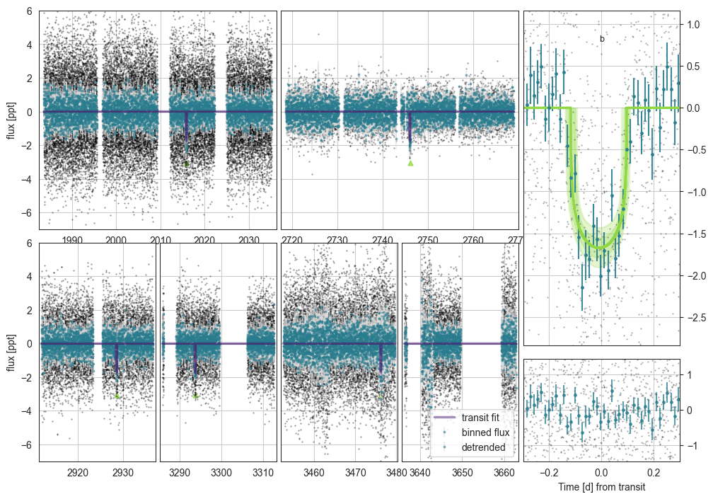
Lightcurve plot
[196]:
mod.plot(plot_flat=True,ylim=(-7,6),xlim=(-0.3,0.3))
initialising transit
Initalising Transit models for plotting with n_samp= 990
0.29085769063688505
E4 - Predicting future transits
By default it looks for the next 6 months:
[208]:
mod.predict_future_transits()
time range 2025-06-05T10:35:57.844 -> 2025-12-02T10:35:57.844
[208]:
| transit_mid_date | transit_mid_med | transit_dur_med | transit_dur_-1sig | transit_dur_+1sig | transit_start_+2sig | transit_start_+1sig | transit_start_med | transit_start_-1sig | transit_start_-2sig | ... | planet_name | alias_n | alias_p | aliases_ns | aliases_ps | total_prob | num_aliases | in_TESS | sun_separation | moon_separation | |
|---|---|---|---|---|---|---|---|---|---|---|---|---|---|---|---|---|---|---|---|---|---|
| 0 | 2025-06-14T19:02:22.380 | 3841.293315 | 0.212578 | 0.197078 | 0.225839 | 3841.220966 | 3841.204607 | 3841.187026 | 3841.171933 | 3841.160183 | ... | duo_b | 0 | 182.546584 | 0,1,2,3,4 | 182.5466,91.2733,60.8489,45.6366,36.5093 | 1.000000 | 5.0 | False | 52.544191 | 118.327951 |
| 1 | 2025-07-21T07:15:48.020 | 3877.802639 | 0.212578 | 0.197078 | 0.225839 | 3877.731026 | 3877.714099 | 3877.696350 | 3877.681083 | 3877.669042 | ... | duo_b | 4 | 36.509317 | 4 | 36.5093 | 0.367791 | 1.0 | False | 62.345520 | 47.477300 |
| 2 | 2025-07-30T10:19:09.864 | 3886.929975 | 0.212578 | 0.197078 | 0.225839 | 3886.858507 | 3886.841483 | 3886.823686 | 3886.808382 | 3886.796219 | ... | duo_b | 3 | 45.636646 | 3 | 45.6366 | 0.289220 | 1.0 | False | 66.518755 | 107.544954 |
| 3 | 2025-08-14T15:24:46.121 | 3902.142200 | 0.212578 | 0.197078 | 0.225839 | 3902.070824 | 3902.053826 | 3902.035912 | 3902.020549 | 3902.008190 | ... | duo_b | 2 | 60.848861 | 2 | 60.8489 | 0.205339 | 1.0 | False | 74.395310 | 62.280802 |
| 4 | 2025-08-26T19:29:18.326 | 3914.312018 | 0.212578 | 0.197078 | 0.225839 | 3914.240677 | 3914.223660 | 3914.205729 | 3914.190277 | 3914.177786 | ... | duo_b | 4 | 36.509317 | 4 | 36.5093 | 0.367791 | 1.0 | False | 81.262697 | 107.927690 |
| 5 | 2025-09-14T01:36:01.307 | 3932.566682 | 0.212578 | 0.197078 | 0.225839 | 3932.495460 | 3932.478442 | 3932.460393 | 3932.444825 | 3932.432142 | ... | duo_b | 1 | 91.273292 | 1,3 | 91.2733,45.6366 | 0.411575 | 2.0 | False | 92.017277 | 47.053472 |
| 6 | 2025-10-02T07:42:45.018 | 3950.821354 | 0.212578 | 0.197078 | 0.225839 | 3950.750449 | 3950.733243 | 3950.715066 | 3950.699338 | 3950.686588 | ... | duo_b | 4 | 36.509317 | 4 | 36.5093 | 0.367791 | 1.0 | False | 102.752449 | 117.097146 |
| 7 | 2025-10-14T11:47:14.205 | 3962.991137 | 0.212578 | 0.197078 | 0.225839 | 3962.920469 | 3962.903098 | 3962.884848 | 3962.869048 | 3962.856144 | ... | duo_b | 2 | 60.848861 | 2 | 60.8489 | 0.205339 | 1.0 | False | 109.542422 | 59.746670 |
| 8 | 2025-10-29T16:52:50.382 | 3978.203361 | 0.212578 | 0.197078 | 0.225839 | 3978.132993 | 3978.115408 | 3978.097072 | 3978.081168 | 3978.068057 | ... | duo_b | 3 | 45.636646 | 3 | 45.6366 | 0.289220 | 1.0 | False | 117.160653 | 116.725954 |
| 9 | 2025-11-07T19:56:11.882 | 3987.330693 | 0.212578 | 0.197078 | 0.225839 | 3987.260508 | 3987.242770 | 3987.224404 | 3987.208457 | 3987.195162 | ... | duo_b | 4 | 36.509317 | 4 | 36.5093 | 0.367791 | 1.0 | False | 121.013362 | 47.249288 |
10 rows × 30 columns
[209]:
df = mod.make_table()
df
Saving sampled model parameters to file with shape: (9314, 14)
[209]:
| mean | sd | hdi_3% | hdi_97% | mcse_mean | mcse_sd | ess_bulk | ess_tail | r_hat | 5% | -$1\sigma$ | median | +$1\sigma$ | 95% | |
|---|---|---|---|---|---|---|---|---|---|---|---|---|---|---|
| Rs | 0.75903 | 0.04050 | 0.68584 | 0.83318 | 0.00316 | 0.00224 | 171.01372 | 579.84759 | 1.03478 | 0.69107 | 0.71511 | 0.76219 | 0.79868 | 0.82463 |
| rhostar | 2.33074 | 0.43892 | 1.52493 | 3.12482 | 0.04886 | 0.03497 | 81.43689 | 167.81385 | 1.07551 | 1.58759 | 1.86375 | 2.34572 | 2.77562 | 3.04480 |
| t0_b[0] | 2015.82597 | 0.00735 | 2015.81237 | 2015.83956 | 0.00125 | 0.00089 | 36.28396 | 247.07322 | 1.14869 | 2015.81376 | 2015.81873 | 2015.82557 | 2015.83394 | 2015.83783 |
| t0_b[1] | 2746.05598 | 0.02272 | 2746.01700 | 2746.09961 | 0.00372 | 0.00265 | 37.89330 | 95.03845 | 1.11385 | 2746.01937 | 2746.03170 | 2746.05707 | 2746.07950 | 2746.09370 |
| t0_b[2] | 2928.55699 | 0.02090 | 2928.51941 | 2928.59772 | 0.00187 | 0.00133 | 125.70602 | 296.18575 | 1.02444 | 2928.52335 | 2928.53611 | 2928.55628 | 2928.57823 | 2928.59301 |
| ... | ... | ... | ... | ... | ... | ... | ... | ... | ... | ... | ... | ... | ... | ... |
| ecc_marg_av_b | 0.30971 | 0.16610 | 0.07270 | 0.65055 | 0.04126 | 0.02971 | 15.81982 | 34.17540 | 1.32507 | 0.12329 | 0.14933 | 0.24883 | 0.42684 | 0.67428 |
| ecc_marg_sd_b | 0.01365 | 0.00895 | 0.00419 | 0.03019 | 0.00196 | 0.00141 | 18.67613 | 82.13914 | 1.22990 | 0.00507 | 0.00702 | 0.01110 | 0.02029 | 0.03148 |
| vel_marg_b | 0.83900 | 0.17135 | 0.45918 | 1.10454 | 0.04475 | 0.03336 | 14.32403 | 34.47314 | 1.37040 | 0.48740 | 0.71350 | 0.88434 | 1.00367 | 1.06360 |
| per_marg_av_b | 56.07264 | 7.93798 | 40.63602 | 68.56733 | 2.07976 | 1.50111 | 13.54872 | 78.48915 | 1.39225 | 41.87952 | 46.59363 | 56.45058 | 62.43775 | 68.64177 |
| per_marg_sd_b | 1056.02463 | 884.80687 | 73.11456 | 2713.21873 | 251.40179 | 182.13025 | 12.32250 | 71.14970 | 1.46362 | 149.00842 | 188.08279 | 852.28493 | 1894.09121 | 2830.57632 |
9314 rows × 14 columns
E4 - Making a CHEOPS OR
Useful for me. Probably less useful for you.
[214]:
mod.make_cheops_OR(observe_sigma=6)
INFO: Query finished. [astroquery.utils.tap.core]
time range 2025-08-22T01:12:28.706 -> 2026-02-18T01:12:28.706
SNR for whole transit is:  22.21439642371073
SNR for single orbit in/egress is:  8.887763520815888
2
3
4
Run the following command in a terminal to generate ORs:
"make_xml_files /Users/hugh/Postdoc/MonoTools_working/TIC00103095888/TIC00103095888_2025-06-04_3_output_ORs.csv --auto-expose -f"
[214]:
| ObsReqName | Target | _RAJ2000 | _DEJ2000 | pmra | pmdec | parallax | SpTy | Gmag | dr2_g_mag | ... | N_Visits | Priority | MinEffDur | Gaia_DR2 | BJD_0 | Period | Ph_late | Ph_early | Old_T_eff | N_Ranges | |
|---|---|---|---|---|---|---|---|---|---|---|---|---|---|---|---|---|---|---|---|---|---|
| 0 | TIC103095888_b_period60;85_prob0.20 | TIC103095888 | 4:04:32.60347091 | 74:32:17.3872212 | -37.019048 | 12.694132 | 7.31134 | G9 | 11.461562 | 11.461562 | ... | 1 | 2 | 45 | 549939402265939072 | 2460476.199873 | 60.848861 | 0.997126 | 0.995548 | -99.0 | 0 |
| 1 | TIC103095888_b_period45;64_prob0.28 | TIC103095888 | 4:04:32.60347091 | 74:32:17.3872212 | -37.019048 | 12.694132 | 7.31134 | G9 | 11.461562 | 11.461562 | ... | 1 | 2 | 45 | 549939402265939072 | 2460476.199873 | 45.636646 | 0.996168 | 0.994064 | -99.0 | 0 |
| 2 | TIC103095888_b_period36;51_prob0.36 | TIC103095888 | 4:04:32.60347091 | 74:32:17.3872212 | -37.019048 | 12.694132 | 7.31134 | G9 | 11.461562 | 11.461562 | ... | 1 | 1 | 45 | 549939402265939072 | 2460476.199873 | 36.509317 | 0.99521 | 0.99258 | -99.0 | 0 |
3 rows × 28 columns