Example 3 - Modelling an ambiguous transit signal
Here we have a lightcurve with five transits but no clear unique period. Let’s walk through a simple fitting excercise:
[1]:
import numpy as np
import pandas as pd
import os
import arviz as az

from MonoTools.MonoTools import fit, tools, lightcurve
WARNING (pytensor.tensor.blas): Using NumPy C-API based implementation for BLAS functions.
E3 - Downloading the lightcurve
Let’s download the target lightcurve using the attached lightcurve module
[2]:
tic=103095888
lc=lightcurve.multilc(tic,'tess',save=False)
Getting all IDs
Accessing online catalogues to match ID to RA/Dec (may be slow) mission= tess
92 90
Sector 92 not (yet) found on MAST | RESPONCE:404
['/Users/hugh/Postdoc/MonoTools_working/TIC00103095888/orbit-45_qlplc.h5', '/Users/hugh/Postdoc/MonoTools_working/TIC00103095888/orbit-46_qlplc.h5']
['/Users/hugh/Postdoc/MonoTools_working/TIC00103095888/orbit-165_qlplc.h5', '/Users/hugh/Postdoc/MonoTools_working/TIC00103095888/orbit-166_qlplc.h5']
['/Users/hugh/Postdoc/MonoTools_working/TIC00103095888/orbit-179_qlplc.h5', '/Users/hugh/Postdoc/MonoTools_working/TIC00103095888/orbit-180_qlplc.h5']
None
[4]:
lc.remove_binned_arrs()
lc.plot(timeseries=['flux'],plot_ephem={'b':{'p':(2746.02021-2015.81701)/4,'t0':2746.02021},
                    'b2':{'p':(2746.02021-2015.81701)/8,'t0':2746.02021},
                    'b3':{'p':(2746.02021-2015.81701)/20,'t0':2746.02021}},savepng=False)
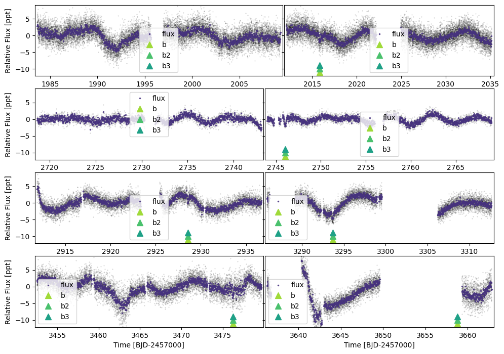
Cleaning up
Due to some scattered light, there’s a couple of very noise regions, which we can mask by updating the lc.mask array:
(In fact, these are pre-removed on the above plot)
[3]:
lc.mask[abs(lc.time-3654.5)<4.8]=False
lc.mask[abs(lc.time-3638.5)<1.75]=False
E3 - Initialising the ambiguous period model
Here, let’s start the model using the TIC id, and passing it the mission (tess) and the lightcurve from above.
We can also initialise the stellar parameters. Without any argument, it uses the TICv8 parameters from the TESS Input Catalogue and stored in the lc class.
We can also initialise the planet. Here we use add_ambiguous as it is a planet with multiple transits, but an ambiguous period. Other options are add_multi (for a normal planet with multiple transits), add_mono (for a single transit) and add_duo (for the unique case of an ambiguous period due to two transits).
To add the planets, you typically need to provide the transit time (or times), the duration (tdur) and the depth (as a ratio).
[35]:
mod = fit.monoModel(tic, 'tess', lc=lc)
mod.init_starpars()
mod.add_ambiguous({'tcens':[2015.81701,
                            np.random.normal(2746.02021,0.015),
                            np.random.normal(2928.57101,0.015),
                            np.random.normal(3293.67261,0.015),
                            3476.22341],
                   'tdur':10/48,'depth':1.8e-3},'b')
{'tcens': array([2015.81701   , 2746.03670605, 2928.5610425 , 3293.66789473,
       3476.22341   ]), 'tdur': 0.20833333333333334, 'depth': 0.0018, 'span': 1460.4064, 'maxperiod_pair': 1, 'maxperiod': 182.5508, 'p_ratios': array([[[ 8., 16., 24., 32., 40., 48., 56., 64., 72., 80., 88., 96.],
        [ 4.,  8., 12., 16., 20., 24., 28., 32., 36., 40., 44., 48.]],

       [[ 8., 16., 24., 32., 40., 48., 56., 64., 72., 80., 88., 96.],
        [ 5., 10., 15., 20., 25., 30., 35., 40., 45., 50., 55., 60.]],

       [[ 8., 16., 24., 32., 40., 48., 56., 64., 72., 80., 88., 96.],
        [ 7., 14., 21., 28., 35., 42., 49., 56., 63., 70., 77., 84.]],

       [[ 8., 16., 24., 32., 40., 48., 56., 64., 72., 80., 88., 96.],
        [ 8., 16., 24., 32., 40., 48., 56., 64., 72., 80., 88., 96.]]]), 'period': 182.5508, 'period_err': 0.034708333333333334, 'period_int_aliases': array([ 8., 16., 24., 32., 40.])}
E3 - Initialising the lightcurve without GPs
There are two main options - with or without a Gaussian Process.
Without a Gaussian Process (use_GP=False) will use a bspline-fitting method (masking the identified transits). This will be faster, but in cases with relatively high-amplitude noise/stellar activity close in duration to the transit, a GP will be more robust. In this case, we do not need all of the data, so we can cut the out-of-transit data, here to 2.5 transit durations from t0, using cut_distance=2.5.
In the case of use_GP=True, bin_oot=True allows for photometry far-from-transit to be binned in order to speed up computation time. Alternatively, bin_all=True will bin all the data including in-transit points. Alternatively fit_no_flatten=True will not perform any flattening and assume the lightcurve is already flat with out-of-transit flux at ~0.0.
[36]:
mod.init_lc(use_GP=False, bin_oot=False, cut_distance=2.5)
[1983.62416643 1996.90862852 2718.63204381 2910.26369667 3285.79832652
 3306.19398793 3452.5326003  3636.2596023 ] [1995.6308658  2035.13108161 2768.97249076 2936.68960795 3303.73569416
 3312.64986176 3479.67162956 3662.82915624]
E3 - Initialising the fit
There are many options for model fitting:
constrain_LD=Truewill constrain the limb darkening coefficients to the theoretical valuesld_mult=3. This is the multiplication factor for the theoretical LD params (to account for systematic errors)model_jitter=Truewill model a log jitter term for each lightcurve (split into cadences)model_phot_mean=Truewill model a mean photometric term for each lightcurve (split into cadences)timing_sigma=0.1allows the adjustment of the priors on the t0s. The default is to assume they are known to ±0.1tdur.floattype=np.float64can be adjusted to e.g.np.float32to attempt to speed up the model.step_initialise=Truewill optimize the model in steps, starting with the most sensitive transit parameters. This is preferred.use_L2=False. If set toTrue, the model will fit for unincluded “second light” (i.e. contamination)model_ambig_ttv=False. If set toTrue, the model does not assume a linear ephemeris for these multiple transits, but includes TTVs.
[37]:
mod.init_model(constrain_LD=True,model_jitter=True,model_phot_mean=True)
[1983.62416643 1996.90862852 2718.63204381 2910.26369667 3285.79832652
 3306.19398793 3452.5326003  3636.2596023 ] [1995.6308658  2035.13108161 2768.97249076 2936.68960795 3303.73569416
 3312.64986176 3479.67162956 3662.82915624]
Initialising ~FAST~ MonoTools model.
initialised planet info
Shape.0
Initialised everything. Optimizing
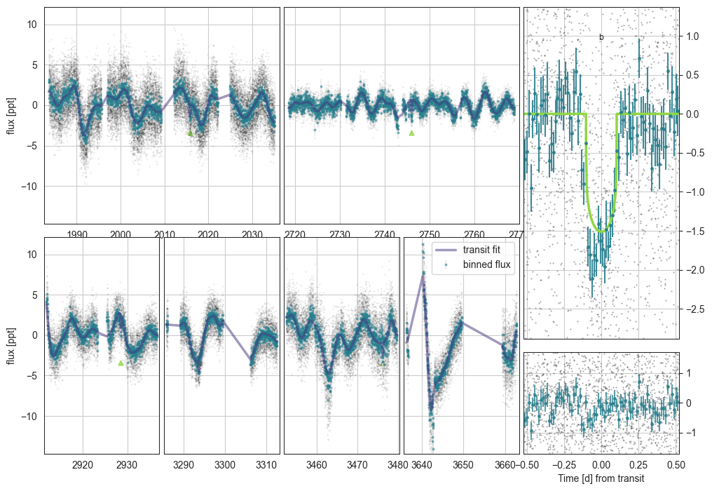
The models are interpolated to the full input lightcurve and stored in mod.trans_to_plot and mod.gp_to_plot.
Additionally, interactive=True may produce an interactive Bokeh plot in the browser.
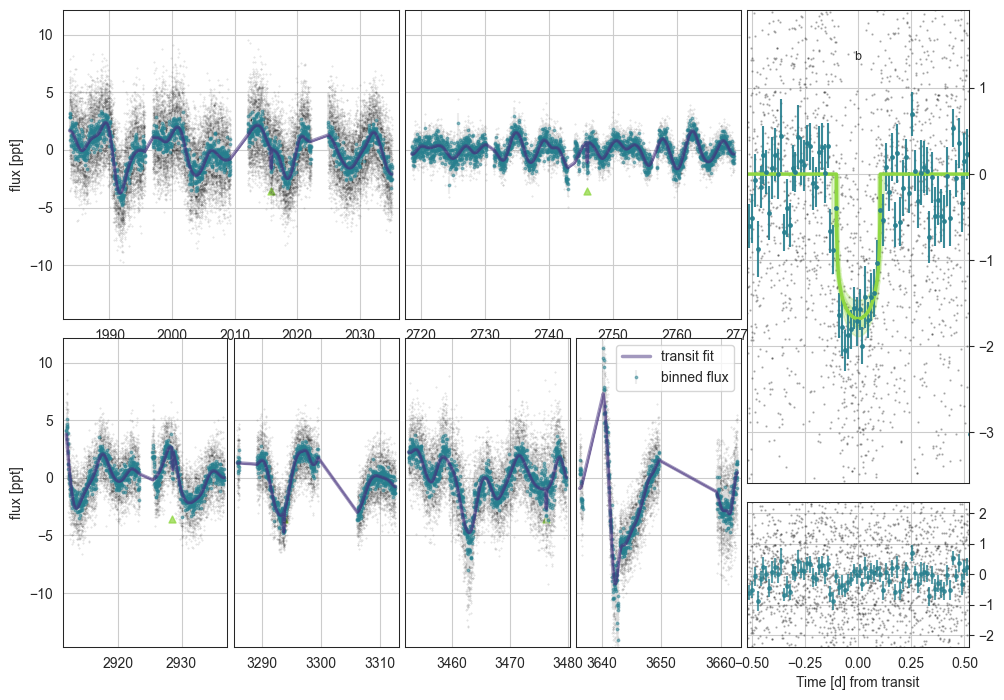
[17]:
mod.plot()
initialising transit
Initalising Transit models for plotting with n_samp= 10
phase (1349,) masked_flux 1349 cad_mask 44161 34000 phasebool (44161,) 1350 transmod (1349,) othpls [0. 0. 0. ... 0. 0. 0.] (1349,)
(726,) (726,) (726,) (726,) (726,)
(1349,) (1349,) (1349,) (1349,) (1349,)
(123,) (123,) (123,) (123,) (123,)
0.34290674778914143
E3 - Sampling the model
The sampling can be modified in the following ways:
n_draws=1800is the number of (post-burn-in) samples per chainn_chains=6is the number of chainscores=6is the number of CPU cores to run on.sample_method=pm.NUTSallows for the ability to run pymc samplers
[56]:
mod.sample_model(overwrite=True,cores=6,n_draws=1800,sample_method=pm.NUTS)
Multiprocess sampling (4 chains in 6 jobs)
NUTS: [Rs, rhostar, t0_b_0, t0_b_4, logror_b, b_b, tdur_b, q_star_tess, log_jitter_ts_120, phot_mean_ts_120, log_jitter_ts_200, phot_mean_ts_200, log_jitter_ts_600, phot_mean_ts_600]
Sampling 4 chains for 1_188 tune and 1_800 draw iterations (4_752 + 7_200 draws total) took 1212 seconds.
Chain 0 reached the maximum tree depth. Increase `max_treedepth`, increase `target_accept` or reparameterize.
Chain 1 reached the maximum tree depth. Increase `max_treedepth`, increase `target_accept` or reparameterize.
Chain 2 reached the maximum tree depth. Increase `max_treedepth`, increase `target_accept` or reparameterize.
Chain 3 reached the maximum tree depth. Increase `max_treedepth`, increase `target_accept` or reparameterize.
The rhat statistic is larger than 1.01 for some parameters. This indicates problems during sampling. See https://arxiv.org/abs/1903.08008 for details
The effective sample size per chain is smaller than 100 for some parameters.  A higher number is needed for reliable rhat and ess computation. See https://arxiv.org/abs/1903.08008 for details
Saving sampled model parameters to file with shape: (27, 14)
Some options are:
Using
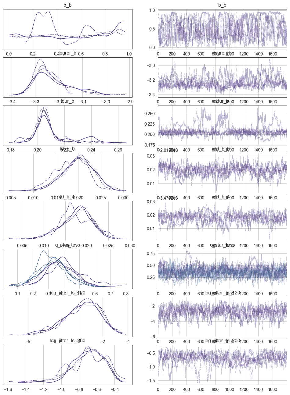
arvizto plot the chainsUsing
mod.plot_cornerto produce corner plots for the planet parametersUsing
mod.plot()
[58]:
_=az.plot_trace(mod.trace['posterior'], var_names=['b_b','logror_b','tdur_b','t0_b_0','t0_b_4','q_star_tess','log_jitter_ts_120','log_jitter_ts_200'])
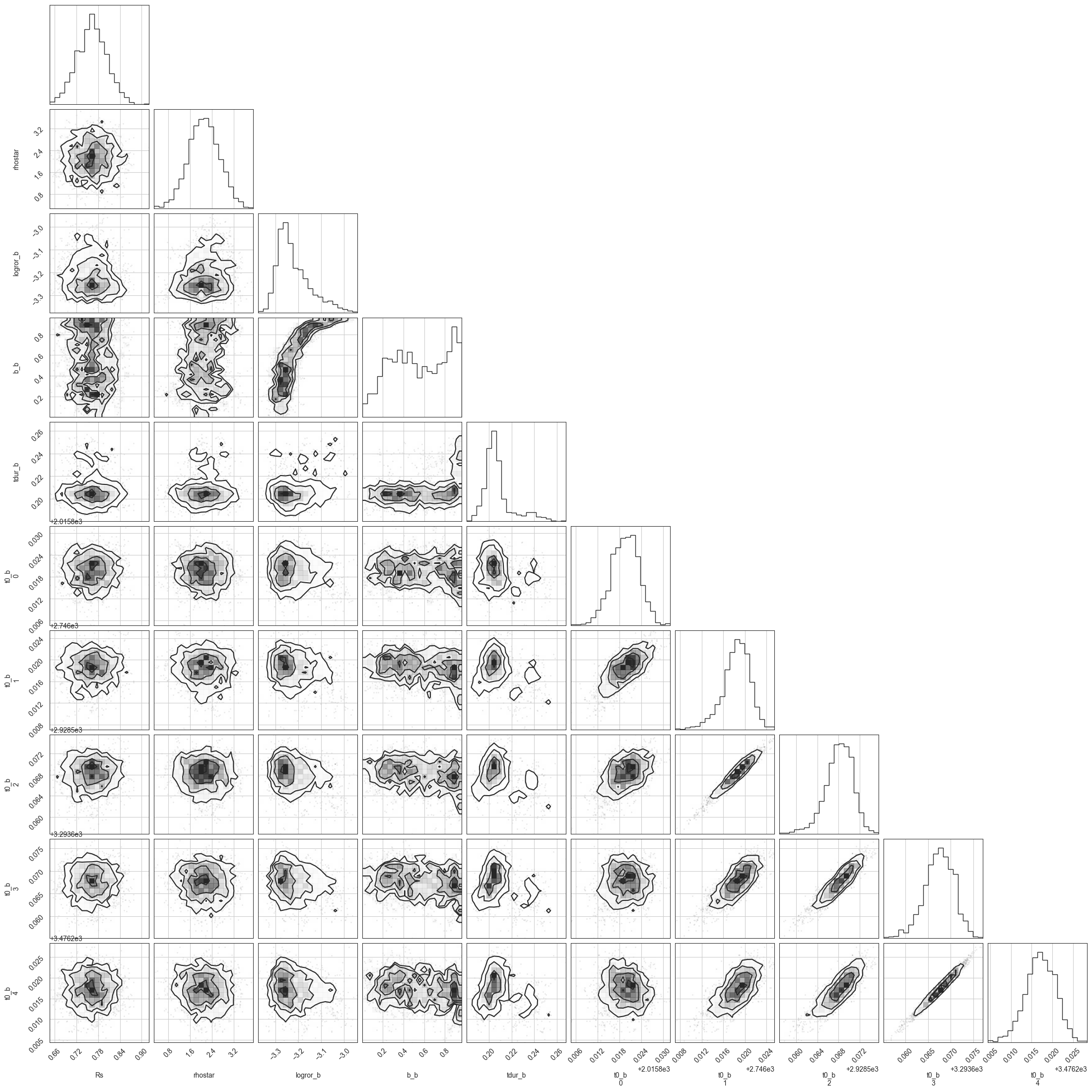
[59]:
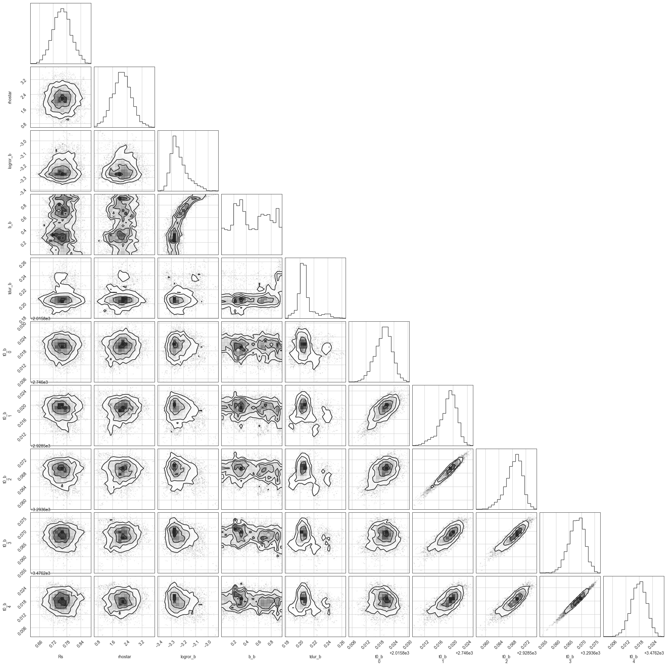
mod.plot_corner()
variables for Corner: ['Rs', 'rhostar', 'logror_b', 'b_b', 'tdur_b', 't0_b']
['Rs', 'rhostar', 'logror_b', 'b_b', 'tdur_b', 't0_b']
[60]:
mod.plot()
initialising transit
Initalising Transit models for plotting with n_samp= 990
phase (1349,) masked_flux 1349 cad_mask 44161 34000 phasebool (44161,) 1350 transmod (1349,) othpls [0. 0. 0. ... 0. 0. 0.] (1349,)
(726,) (726,) (726,) (726,) (726,)
(1349,) (1349,) (1349,) (1349,) (1349,)
(123,) (123,) (123,) (123,) (123,)
0.4763927189622087
E3 - Computing the period probabilities a posteriori
In this new version, we fit the transits in a way ambivalent to the periods, and instead only assess the period probabilities using the trace (and various priors). To do this, you have to call mod.assess_period_from_posterior()
Eccentricity priors
At this point, key choices have to be made about the eccentricity prior by updating ecc_prior='auto'. This is extremely important, as the uncertainty in your derived period distribution depends highly on the eccentricity prior, so choose an option that you believe best matches your planet/planetary system. There are the following options:
ecc_prior='uniform'- Planets don’t have this distribution in reality. Don’t use this.ecc_prior='kipping'- The (close-in) Kipping 2013 prior. Derived from RV planets, and therefore dominated by high-mass planets. Potentially OK in those cases.ecc_prior='vaneylen'- Specifically the multi-planet version derived in VanEylen 2018. Measured for compact multi systems in Kepler. The most e=0-biased prior available (therefore, potentially, the best period logprob constraints)ecc_prior='bernmodel_sing'- Derived from single planets as produced by Bern model full-system simulations. No observational biases. The Bern Model priors are also all radius-dependent using the initial radius to choose one distribution from [terrestrials, Neptunians or Giants]. The giant case matcheskippingwell, while the smaller planets are much more low-eccentricity.ecc_prior='bernmodel_mult'- Derived from multi systems produced by Bern model. Radius-dependent (rocky, Neptunian & Giants). These, especially for small planets, are well-constrained to e~0 (though less so thanvaneylen).ecc_prior='bernmodel_both'- Derived from all (observable) planets as produced by Bern model full-system simulations.ecc_prior='auto'- The default is the (radius-constrained)bernmodel_bothprior for single cases (as we do not know if there could be additional planets), and thebernmodel_multin multi cases.
[61]:
mod.assess_period_from_posterior()
both__bernmodel auto {'kipping': 'kip', 'vaneylen': 'vve', 'flat': 'flat', 'apogee': 'apo', 'bernmodel_both': 'both__bernmodel', 'bernmodel_sing': 'singles__bernmodel', 'bernmodel_mult': 'multis__bernmodel', 'auto': 'both__bernmodel'} both ['bern', 'auto']
E3 - Viewing the derived parameters
mod.make_table() creates (and saves) the posterior statistics. Check that ess is at least a thousand, and r_hat is well below 1.05 (ideally below 1.01).
[62]:
df=mod.make_table()
df.shape
Saving sampled model parameters to file with shape: (84, 14)
[62]:
(84, 14)
[64]:
df.iloc[:42]
[64]:
| mean | sd | hdi_3% | hdi_97% | mcse_mean | mcse_sd | ess_bulk | ess_tail | r_hat | 5% | -$1\sigma$ | median | +$1\sigma$ | 95% | |
|---|---|---|---|---|---|---|---|---|---|---|---|---|---|---|
| Rs | 0.75914 | 0.03932 | 0.68555 | 0.83545 | 0.00245 | 0.00173 | 256.57139 | 554.02383 | 1.01865 | 0.69458 | 0.72013 | 0.75909 | 0.79827 | 0.82624 |
| rhostar | 2.11344 | 0.51435 | 1.10447 | 3.04547 | 0.04724 | 0.03348 | 118.95985 | 376.04896 | 1.03987 | 1.26015 | 1.58644 | 2.11278 | 2.62271 | 2.95344 |
| t0_b_0 | 2015.81954 | 0.00361 | 2015.81227 | 2015.82586 | 0.00033 | 0.00023 | 125.08518 | 257.33884 | 1.02911 | 2015.81328 | 2015.81581 | 2015.81980 | 2015.82304 | 2015.82509 |
| t0_b_4 | 3476.21778 | 0.00349 | 3476.21136 | 3476.22438 | 0.00036 | 0.00026 | 88.44852 | 137.51605 | 1.01490 | 3476.21187 | 3476.21431 | 3476.21795 | 3476.22126 | 3476.22334 |
| logror_b | -3.23370 | 0.07041 | -3.34304 | -3.08708 | 0.00847 | 0.00602 | 63.27842 | 220.54433 | 1.05399 | -3.32226 | -3.29658 | -3.24998 | -3.16546 | -3.09006 |
| tdur_b | 0.20825 | 0.01245 | 0.18952 | 0.24084 | 0.00180 | 0.00128 | 71.90059 | 76.25026 | 1.05726 | 0.19292 | 0.19962 | 0.20544 | 0.21631 | 0.23811 |
| log_jitter_ts_120 | -2.79781 | 0.68822 | -4.13588 | -1.55716 | 0.04692 | 0.03323 | 219.00424 | 406.19278 | 1.00444 | -4.06133 | -3.50086 | -2.73259 | -2.11362 | -1.76882 |
| phot_mean_ts_120 | 0.04083 | 0.06181 | -0.07512 | 0.15919 | 0.00378 | 0.00271 | 264.65389 | 706.43017 | 1.05399 | -0.05565 | -0.02056 | 0.03736 | 0.10405 | 0.14691 |
| log_jitter_ts_200 | -0.70331 | 0.19710 | -1.05629 | -0.38840 | 0.02013 | 0.01428 | 91.36896 | 203.54593 | 1.02845 | -1.02964 | -0.88988 | -0.68422 | -0.50974 | -0.43137 |
| phot_mean_ts_200 | -0.03908 | 0.03345 | -0.10012 | 0.02480 | 0.00245 | 0.00174 | 182.38262 | 595.42982 | 1.03133 | -0.09161 | -0.07126 | -0.04087 | -0.00661 | 0.01730 |
| log_jitter_ts_600 | -2.28692 | 0.80070 | -3.72910 | -0.91801 | 0.08413 | 0.05968 | 87.52678 | 467.01545 | 1.05905 | -3.69317 | -3.13616 | -2.18849 | -1.47273 | -1.13774 |
| phot_mean_ts_600 | -0.33116 | 0.06188 | -0.45383 | -0.22948 | 0.00969 | 0.00690 | 43.40210 | 872.63843 | 1.07932 | -0.43298 | -0.39317 | -0.33082 | -0.26758 | -0.23820 |
| b_b | 0.49610 | 0.27370 | 0.06304 | 0.94508 | 0.03335 | 0.02542 | 81.48908 | 141.66965 | 1.03550 | 0.06428 | 0.20416 | 0.47808 | 0.81933 | 0.92315 |
| q_star_tess[0] | 0.38437 | 0.10744 | 0.16907 | 0.57045 | 0.00960 | 0.00753 | 146.11450 | 129.28704 | 1.03513 | 0.21667 | 0.28182 | 0.37794 | 0.48451 | 0.56682 |
| q_star_tess[1] | 0.32718 | 0.09439 | 0.16521 | 0.52269 | 0.00635 | 0.00449 | 219.68283 | 419.05766 | 1.02973 | 0.18072 | 0.23537 | 0.32579 | 0.41813 | 0.48949 |
| t0_b_1 | 2746.01866 | 0.00244 | 2746.01366 | 2746.02293 | 0.00028 | 0.00020 | 81.68791 | 152.66514 | 1.01201 | 2746.01387 | 2746.01630 | 2746.01900 | 2746.02094 | 2746.02206 |
| t0_b_2 | 2928.56844 | 0.00250 | 2928.56348 | 2928.57293 | 0.00029 | 0.00021 | 75.62354 | 161.53714 | 1.01061 | 2928.56368 | 2928.56602 | 2928.56877 | 2928.57082 | 2928.57196 |
| t0_b_3 | 3293.66800 | 0.00306 | 3293.66178 | 3293.67321 | 0.00033 | 0.00024 | 81.21301 | 142.36871 | 1.01613 | 3293.66279 | 3293.66492 | 3293.66821 | 3293.67101 | 3293.67265 |
| t0_b[0] | 2015.81954 | 0.00361 | 2015.81227 | 2015.82586 | 0.00033 | 0.00023 | 125.08518 | 257.33884 | 1.02911 | 2015.81328 | 2015.81581 | 2015.81980 | 2015.82304 | 2015.82509 |
| t0_b[1] | 2746.01866 | 0.00244 | 2746.01366 | 2746.02293 | 0.00028 | 0.00020 | 81.68791 | 152.66514 | 1.01201 | 2746.01387 | 2746.01630 | 2746.01900 | 2746.02094 | 2746.02206 |
| t0_b[2] | 2928.56844 | 0.00250 | 2928.56348 | 2928.57293 | 0.00029 | 0.00021 | 75.62354 | 161.53714 | 1.01061 | 2928.56368 | 2928.56602 | 2928.56877 | 2928.57082 | 2928.57196 |
| t0_b[3] | 3293.66800 | 0.00306 | 3293.66178 | 3293.67321 | 0.00033 | 0.00024 | 81.21301 | 142.36871 | 1.01613 | 3293.66279 | 3293.66492 | 3293.66821 | 3293.67101 | 3293.67265 |
| t0_b[4] | 3476.21778 | 0.00349 | 3476.21136 | 3476.22438 | 0.00036 | 0.00026 | 88.44852 | 137.51605 | 1.01490 | 3476.21187 | 3476.21431 | 3476.21795 | 3476.22126 | 3476.22334 |
| ror_b | 0.03951 | 0.00289 | 0.03529 | 0.04559 | 0.00035 | 0.00024 | 63.27842 | 220.54433 | 1.05399 | 0.03607 | 0.03701 | 0.03877 | 0.04219 | 0.04550 |
| rpl_b | 3.27649 | 0.30660 | 2.74455 | 3.87948 | 0.03424 | 0.02430 | 79.34175 | 256.33372 | 1.05196 | 2.86053 | 2.98747 | 3.23042 | 3.56464 | 3.87111 |
| u_star_tess[0] | 0.40177 | 0.12886 | 0.17228 | 0.65084 | 0.00868 | 0.00614 | 219.57597 | 504.96780 | 1.01664 | 0.20463 | 0.27272 | 0.39428 | 0.52889 | 0.62576 |
| u_star_tess[1] | 0.21205 | 0.11955 | -0.02478 | 0.42153 | 0.00934 | 0.00661 | 163.05266 | 520.12065 | 1.02107 | 0.01265 | 0.09459 | 0.21158 | 0.33188 | 0.40455 |
| pcirc_b | 0.00000 | 0.00000 | 0.00000 | 0.00000 | 0.00000 | 0.00000 | 70.98957 | 103.95803 | 1.03879 | 0.00000 | 0.00000 | 0.00000 | 0.00000 | 0.00000 |
| per_b[0] | 182.54978 | 0.00065 | 182.54860 | 182.55105 | 0.00005 | 0.00003 | 171.82602 | 391.00644 | 1.02377 | 182.54868 | 182.54915 | 182.54980 | 182.55042 | 182.55086 |
| per_b[1] | 91.27489 | 0.00032 | 91.27430 | 91.27552 | 0.00002 | 0.00002 | 171.82602 | 391.00644 | 1.02377 | 91.27434 | 91.27457 | 91.27490 | 91.27521 | 91.27543 |
| per_b[2] | 60.84993 | 0.00022 | 60.84953 | 60.85035 | 0.00002 | 0.00001 | 171.82602 | 391.00644 | 1.02377 | 60.84956 | 60.84972 | 60.84993 | 60.85014 | 60.85029 |
| per_b[3] | 45.63744 | 0.00016 | 45.63715 | 45.63776 | 0.00001 | 0.00001 | 171.82602 | 391.00644 | 1.02377 | 45.63717 | 45.63729 | 45.63745 | 45.63761 | 45.63772 |
| per_b[4] | 36.50996 | 0.00013 | 36.50972 | 36.51021 | 0.00001 | 0.00001 | 171.82602 | 391.00644 | 1.02377 | 36.50974 | 36.50983 | 36.50996 | 36.51008 | 36.51017 |
| av_t0_b | 3476.21778 | 0.00349 | 3476.21136 | 3476.22438 | 0.00036 | 0.00026 | 88.44852 | 137.51605 | 1.01490 | 3476.21187 | 3476.21431 | 3476.21795 | 3476.22126 | 3476.22334 |
| vel_b[0] | 1.40417 | 0.35531 | 0.62596 | 1.93805 | 0.05002 | 0.03578 | 49.31916 | 126.64398 | 1.07962 | 0.72507 | 1.02382 | 1.45045 | 1.73029 | 1.92521 |
| vel_b[1] | 1.11449 | 0.28201 | 0.49683 | 1.53823 | 0.03970 | 0.02840 | 49.31916 | 126.64398 | 1.07962 | 0.57549 | 0.81260 | 1.15123 | 1.37334 | 1.52804 |
| vel_b[2] | 0.97360 | 0.24636 | 0.43402 | 1.34377 | 0.03469 | 0.02481 | 49.31916 | 126.64398 | 1.07962 | 0.50273 | 0.70988 | 1.00569 | 1.19972 | 1.33486 |
| vel_b[3] | 0.88457 | 0.22383 | 0.39433 | 1.22089 | 0.03151 | 0.02254 | 49.31916 | 126.64398 | 1.07962 | 0.45676 | 0.64496 | 0.91373 | 1.09002 | 1.21281 |
| vel_b[4] | 0.82116 | 0.20779 | 0.36607 | 1.13338 | 0.02925 | 0.02093 | 49.31916 | 126.64398 | 1.07962 | 0.42402 | 0.59873 | 0.84823 | 1.01188 | 1.12587 |
| min_ecc_b[0] | 0.34886 | 0.15695 | 0.03158 | 0.59047 | 0.01936 | 0.01444 | 61.44395 | 138.89177 | 1.05594 | 0.06010 | 0.16542 | 0.37242 | 0.50117 | 0.57511 |
| min_ecc_b[1] | 0.23284 | 0.14870 | 0.00010 | 0.50054 | 0.01541 | 0.01093 | 97.61141 | 151.88374 | 1.01944 | 0.02155 | 0.07401 | 0.22089 | 0.37994 | 0.51996 |
| min_ecc_b[2] | 0.20269 | 0.17061 | 0.00010 | 0.57371 | 0.01709 | 0.01277 | 125.66511 | 126.64398 | 1.02749 | 0.01430 | 0.04998 | 0.15409 | 0.36035 | 0.59650 |
[66]:
df.iloc[42:]
[66]:
| mean | sd | hdi_3% | hdi_97% | mcse_mean | mcse_sd | ess_bulk | ess_tail | r_hat | 5% | -$1\sigma$ | median | +$1\sigma$ | 95% | |
|---|---|---|---|---|---|---|---|---|---|---|---|---|---|---|
| min_ecc_b[3] | 0.21145 | 0.19519 | 0.00010 | 0.63451 | 0.02044 | 0.01549 | 124.39393 | 126.64398 | 1.04204 | 0.01330 | 0.03818 | 0.14673 | 0.41299 | 0.65476 |
| min_ecc_b[4] | 0.24113 | 0.20948 | 0.00010 | 0.67686 | 0.02569 | 0.01824 | 76.78674 | 126.64398 | 1.04760 | 0.01379 | 0.04555 | 0.17595 | 0.47223 | 0.69521 |
| omega_b[0] | 2.03374 | 1.11366 | 1.57080 | 4.71239 | 0.11966 | 0.08490 | 86.61159 | 86.61159 | 1.04865 | 1.57080 | 1.57080 | 1.57080 | 1.57080 | 4.71239 |
| omega_b[1] | 2.55996 | 1.45925 | 1.57080 | 4.71239 | 0.15679 | 0.11124 | 86.62023 | 86.62023 | 1.04477 | 1.57080 | 1.57080 | 1.57080 | 4.71239 | 4.71239 |
| omega_b[2] | 3.11236 | 1.57063 | 1.57080 | 4.71239 | 0.18873 | 0.13402 | 69.25912 | 69.25912 | 1.04583 | 1.57080 | 1.57080 | 1.57080 | 4.71239 | 4.71239 |
| omega_b[3] | 3.64774 | 1.48712 | 1.57080 | 4.71239 | 0.19192 | 0.13637 | 60.04177 | 60.04177 | 1.05496 | 1.57080 | 1.57080 | 4.71239 | 4.71239 | 4.71239 |
| omega_b[4] | 4.14298 | 1.21030 | 1.57080 | 4.71239 | 0.14629 | 0.10389 | 68.44742 | 68.44742 | 1.04141 | 1.57080 | 1.57080 | 4.71239 | 4.71239 | 4.71239 |
| perprior_b[0] | -4.29182 | 0.00001 | -4.29184 | -4.29180 | 0.00000 | 0.00000 | 171.82602 | 391.00644 | 1.02377 | -4.29184 | -4.29183 | -4.29182 | -4.29181 | -4.29180 |
| perprior_b[1] | -2.44343 | 0.00001 | -2.44345 | -2.44341 | 0.00000 | 0.00000 | 171.82602 | 391.00644 | 1.02377 | -2.44344 | -2.44344 | -2.44343 | -2.44342 | -2.44341 |
| perprior_b[2] | -1.36219 | 0.00001 | -1.36221 | -1.36217 | 0.00000 | 0.00000 | 171.82602 | 391.00644 | 1.02377 | -1.36220 | -1.36220 | -1.36219 | -1.36218 | -1.36217 |
| perprior_b[3] | -0.59503 | 0.00001 | -0.59505 | -0.59502 | 0.00000 | 0.00000 | 171.82602 | 391.00644 | 1.02377 | -0.59505 | -0.59504 | -0.59503 | -0.59503 | -0.59502 |
| perprior_b[4] | 0.00001 | 0.00001 | -0.00000 | 0.00003 | 0.00000 | 0.00000 | 171.82602 | 391.00644 | 1.02377 | -0.00000 | 0.00001 | 0.00001 | 0.00002 | 0.00003 |
| a_Rs_b[0] | 172.52811 | 14.68593 | 142.80758 | 198.24991 | 1.32979 | 0.95198 | 118.96160 | 376.04896 | 1.03987 | 146.24238 | 157.90852 | 173.73269 | 186.71627 | 194.25599 |
| a_Rs_b[1] | 108.68590 | 9.25156 | 89.96314 | 124.88961 | 0.83772 | 0.59971 | 118.96160 | 376.04896 | 1.03987 | 92.12692 | 99.47613 | 109.44474 | 117.62388 | 122.37360 |
| a_Rs_b[2] | 82.94286 | 7.06026 | 68.65472 | 95.30861 | 0.63930 | 0.45766 | 118.96160 | 376.04896 | 1.03987 | 70.30600 | 75.91450 | 83.52197 | 89.76382 | 93.38854 |
| a_Rs_b[3] | 68.46782 | 5.82812 | 56.67323 | 78.67553 | 0.52773 | 0.37779 | 118.96160 | 376.04896 | 1.03987 | 58.03633 | 62.66604 | 68.94586 | 74.09840 | 77.09054 |
| a_Rs_b[4] | 59.00378 | 5.02252 | 48.83951 | 67.80051 | 0.45478 | 0.32557 | 118.96160 | 376.04896 | 1.03987 | 50.01419 | 54.00395 | 59.41574 | 63.85607 | 66.43461 |
| max_ecc_b[0] | 0.98832 | 0.00107 | 0.98633 | 0.99014 | 0.00009 | 0.00007 | 118.96160 | 376.04896 | 1.03987 | 0.98632 | 0.98733 | 0.98849 | 0.98929 | 0.98970 |
| max_ecc_b[1] | 0.98146 | 0.00170 | 0.97830 | 0.98435 | 0.00015 | 0.00010 | 118.96160 | 376.04896 | 1.03987 | 0.97829 | 0.97989 | 0.98173 | 0.98300 | 0.98366 |
| max_ecc_b[2] | 0.97570 | 0.00222 | 0.97156 | 0.97949 | 0.00019 | 0.00014 | 118.96160 | 376.04896 | 1.03987 | 0.97155 | 0.97365 | 0.97605 | 0.97772 | 0.97858 |
| max_ecc_b[3] | 0.97056 | 0.00269 | 0.96555 | 0.97516 | 0.00023 | 0.00017 | 118.96160 | 376.04896 | 1.03987 | 0.96554 | 0.96808 | 0.97099 | 0.97301 | 0.97406 |
| max_ecc_b[4] | 0.96584 | 0.00312 | 0.96003 | 0.97117 | 0.00027 | 0.00019 | 118.96160 | 376.04896 | 1.03987 | 0.96001 | 0.96297 | 0.96634 | 0.96868 | 0.96990 |
| vprior_b[0] | -0.80963 | 0.67794 | -2.03887 | 0.61117 | 0.05995 | 0.04633 | 112.72127 | 203.78813 | 1.02524 | -1.85743 | -1.42358 | -0.89115 | -0.13742 | 0.44053 |
| vprior_b[1] | -0.53961 | 0.91935 | -2.73291 | 1.00090 | 0.09229 | 0.06900 | 112.15321 | 125.87980 | 1.02277 | -2.58502 | -1.26731 | -0.39979 | 0.22668 | 0.71273 |
| vprior_b[2] | -0.62348 | 1.15426 | -3.21413 | 1.08145 | 0.11578 | 0.09425 | 133.56312 | 125.87980 | 1.05781 | -3.10180 | -1.83558 | -0.31052 | 0.38205 | 0.80434 |
| vprior_b[3] | -0.85872 | 1.30256 | -3.60351 | 1.05611 | 0.15558 | 0.11047 | 81.39631 | 125.87980 | 1.04252 | -3.45485 | -2.24006 | -0.63246 | 0.42993 | 0.82800 |
| vprior_b[4] | -1.19028 | 1.31706 | -3.78369 | 1.11542 | 0.17721 | 0.12598 | 57.72708 | 125.87980 | 1.06242 | -3.72745 | -2.53756 | -1.08251 | 0.16478 | 0.72859 |
| logprob_b[0] | -6714.16475 | 2.38734 | -6718.83192 | -6709.96759 | 0.17272 | 0.12232 | 187.32511 | 928.24080 | 1.00852 | -6718.39345 | -6716.47569 | -6713.99500 | -6711.83263 | -6710.59127 |
| logprob_b[1] | -6712.04634 | 2.43406 | -6716.73606 | -6707.88305 | 0.17835 | 0.12631 | 184.88546 | 712.45872 | 1.00607 | -6716.45288 | -6714.49939 | -6711.78558 | -6709.64667 | -6708.45203 |
| logprob_b[2] | -6711.04897 | 2.51133 | -6715.90412 | -6706.62250 | 0.17500 | 0.12392 | 210.51945 | 609.26881 | 1.01667 | -6715.63719 | -6713.52885 | -6710.79440 | -6708.58824 | -6707.42172 |
| logprob_b[3] | -6710.51706 | 2.56678 | -6715.69232 | -6706.23892 | 0.18162 | 0.12861 | 202.98184 | 566.56674 | 1.02609 | -6715.20049 | -6713.02120 | -6710.26241 | -6708.00307 | -6706.79203 |
| logprob_b[4] | -6710.25357 | 2.55079 | -6715.15222 | -6705.63762 | 0.18943 | 0.13417 | 180.85984 | 525.43579 | 1.02672 | -6714.85210 | -6712.76079 | -6710.00212 | -6707.79130 | -6706.48994 |
| ecc_b[0] | 0.48466 | 0.17166 | 0.12100 | 0.73682 | 0.02146 | 0.01638 | 56.10927 | 146.88106 | 1.06250 | 0.14757 | 0.29180 | 0.52208 | 0.64619 | 0.70956 |
| ecc_b[1] | 0.35902 | 0.16374 | 0.04555 | 0.63095 | 0.01740 | 0.01244 | 93.51210 | 263.70869 | 1.02068 | 0.08555 | 0.16880 | 0.36980 | 0.53137 | 0.62696 |
| ecc_b[2] | 0.31054 | 0.17227 | 0.03350 | 0.65242 | 0.01671 | 0.01239 | 118.97314 | 129.07275 | 1.01785 | 0.07180 | 0.13622 | 0.28327 | 0.48579 | 0.66113 |
| ecc_b[3] | 0.30582 | 0.19135 | 0.03735 | 0.70917 | 0.01866 | 0.01437 | 130.43431 | 126.64398 | 1.03782 | 0.06997 | 0.11911 | 0.26486 | 0.50812 | 0.71069 |
| ecc_b[4] | 0.32970 | 0.20331 | 0.03484 | 0.74013 | 0.02352 | 0.01703 | 87.27568 | 126.64398 | 1.04238 | 0.07088 | 0.12716 | 0.28364 | 0.55543 | 0.74574 |
| ecc_marg_av_b | 0.28329 | 0.17512 | 0.07252 | 0.68004 | 0.01778 | 0.01332 | 133.69406 | 126.64398 | 1.02903 | 0.11189 | 0.14021 | 0.22851 | 0.43020 | 0.68658 |
| ecc_marg_sd_b | 0.01114 | 0.00675 | 0.00362 | 0.02319 | 0.00037 | 0.00026 | 283.91514 | 1264.14921 | 1.01527 | 0.00478 | 0.00628 | 0.00901 | 0.01577 | 0.02457 |
| vel_marg_b | 0.90226 | 0.20179 | 0.41050 | 1.18413 | 0.02781 | 0.01995 | 49.53510 | 126.64398 | 1.07933 | 0.47677 | 0.71542 | 0.96573 | 1.04469 | 1.17609 |
| per_marg_av_b | 52.17087 | 7.82383 | 40.16136 | 64.05983 | 0.94241 | 0.66923 | 77.30736 | 849.53915 | 1.03951 | 41.37299 | 42.45703 | 53.81017 | 59.11554 | 64.13437 |
| per_marg_sd_b | 710.11117 | 688.85554 | 80.90609 | 1913.96319 | 72.72649 | 51.59351 | 69.05038 | 935.78585 | 1.05149 | 135.43957 | 164.74699 | 347.23598 | 1317.09089 | 2024.44543 |
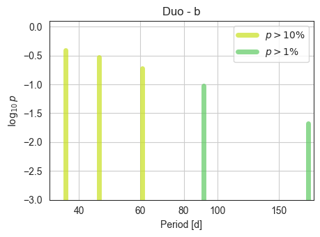
E3 - Plotting the period alias probabilities
[72]:
mod.plot_periods(ymin=-3)
E3 - Saving the model
This will save all class variables in a pickle, and the trace in a .nc file
[73]:
mod.save_model_to_file()
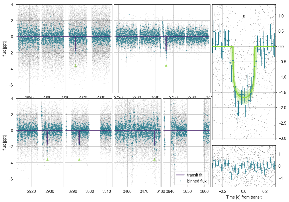
[127]:
mod.plot(overwrite=True, ylim=(-7,4), xlim=(-0.3,0.3), plot_flat=True)
{0: {'start': 1983.6297218556767, 'end': 2035.1310816138769, 'cadname': 'ts_120'}, 1: {'start': 2911.8632512550407, 'end': 2936.6896079470475, 'cadname': 'ts_200'}, 2: {'start': 3285.80295614306, 'end': 3312.649861760622, 'cadname': 'ts_200'}, 3: {'start': 3452.5326002979305, 'end': 3479.6716295550805, 'cadname': 'ts_200'}, 4: {'start': 3636.2596023021974, 'end': 3662.829156239456, 'cadname': 'ts_200'}, 5: {'start': 2718.6389880929823, 'end': 2768.972490764838, 'cadname': 'ts_600'}}
{0: {'start': 1983.6297218556767, 'end': 2035.1310816138769, 'cadname': 'ts_120'}, 5: {'start': 2718.6389880929823, 'end': 2768.972490764838, 'cadname': 'ts_600'}, 1: {'start': 2911.8632512550407, 'end': 2936.6896079470475, 'cadname': 'ts_200'}, 2: {'start': 3285.80295614306, 'end': 3312.649861760622, 'cadname': 'ts_200'}, 3: {'start': 3452.5326002979305, 'end': 3479.6716295550805, 'cadname': 'ts_200'}, 4: {'start': 3636.2596023021974, 'end': 3662.829156239456, 'cadname': 'ts_200'}}
initialising transit
Initalising Transit models for plotting with n_samp= 990
0.34362523743915974
E3 - Predicting future transits
[130]:
mod.predict_future_transits()
time range 2025-05-22T10:27:09.630 -> 2025-11-18T10:27:09.633
[130]:
| transit_mid_date | transit_mid_med | transit_dur_med | transit_dur_-1sig | transit_dur_+1sig | transit_start_+2sig | transit_start_+1sig | transit_start_med | transit_start_-1sig | transit_start_-2sig | ... | planet_name | alias_n | alias_p | aliases_ns | aliases_ps | total_prob | num_aliases | in_TESS | sun_separation | moon_separation | |
|---|---|---|---|---|---|---|---|---|---|---|---|---|---|---|---|---|---|---|---|---|---|
| 0 | 2025-06-14T19:35:56.970 | 3841.316632 | 0.204842 | 0.198116 | 0.215877 | 3841.230801 | 3841.222288 | 3841.214211 | 3841.203897 | 3841.185052 | ... | duo_b | 0 | 182.549693 | 0,1,2,3,4 | 182.5497,91.2748,60.8499,45.6374,36.5099 | 1.000000 | 5.0 | False | 52.545917 | 118.162380 |
| 1 | 2025-07-21T07:50:16.117 | 3877.826575 | 0.204842 | 0.198116 | 0.215877 | 3877.740917 | 3877.732349 | 3877.724155 | 3877.713692 | 3877.694763 | ... | duo_b | 4 | 36.509939 | 4 | 36.5099 | 0.402557 | 1.0 | False | 62.355785 | 47.446337 |
| 2 | 2025-07-30T10:53:51.233 | 3886.954065 | 0.204842 | 0.198116 | 0.215877 | 3886.868444 | 3886.859880 | 3886.851644 | 3886.841121 | 3886.822194 | ... | duo_b | 3 | 45.637423 | 3 | 45.6374 | 0.305821 | 1.0 | False | 66.530400 | 107.730904 |
| 3 | 2025-08-14T15:59:47.930 | 3902.166527 | 0.204842 | 0.198116 | 0.215877 | 3902.081001 | 3902.072394 | 3902.064106 | 3902.053558 | 3902.034599 | ... | duo_b | 2 | 60.849898 | 2 | 60.8499 | 0.213620 | 1.0 | False | 74.408624 | 62.086731 |
| 4 | 2025-08-26T20:04:34.972 | 3914.336516 | 0.204842 | 0.198116 | 0.215877 | 3914.251044 | 3914.242406 | 3914.234095 | 3914.223497 | 3914.204527 | ... | duo_b | 4 | 36.509939 | 4 | 36.5099 | 0.402557 | 1.0 | False | 81.276866 | 108.117816 |
| 5 | 2025-09-14T02:11:44.635 | 3932.591489 | 0.204842 | 0.198116 | 0.215877 | 3932.506126 | 3932.497435 | 3932.489068 | 3932.478400 | 3932.459408 | ... | duo_b | 1 | 91.274847 | 1,3 | 91.2748,45.6374 | 0.378563 | 2.0 | False | 92.032026 | 47.045340 |
| 6 | 2025-10-02T08:18:56.251 | 3950.846484 | 0.204842 | 0.198116 | 0.215877 | 3950.761209 | 3950.752463 | 3950.744064 | 3950.733351 | 3950.714259 | ... | duo_b | 4 | 36.509939 | 4 | 36.5099 | 0.402557 | 1.0 | False | 102.766891 | 116.910797 |
| 7 | 2025-10-14T12:23:44.020 | 3963.016482 | 0.204842 | 0.198116 | 0.215877 | 3962.931264 | 3962.922486 | 3962.914061 | 3962.903287 | 3962.884185 | ... | duo_b | 2 | 60.849898 | 2 | 60.8499 | 0.213620 | 1.0 | False | 109.556050 | 59.926603 |
| 8 | 2025-10-29T17:29:43.320 | 3978.228974 | 0.204842 | 0.198116 | 0.215877 | 3978.143824 | 3978.135002 | 3978.126553 | 3978.115736 | 3978.096591 | ... | duo_b | 3 | 45.637423 | 3 | 45.6374 | 0.305821 | 1.0 | False | 117.172339 | 116.540551 |
| 9 | 2025-11-07T20:33:18.207 | 3987.356461 | 0.204842 | 0.198116 | 0.215877 | 3987.271363 | 3987.262493 | 3987.254040 | 3987.243183 | 3987.224035 | ... | duo_b | 4 | 36.509939 | 4 | 36.5099 | 0.402557 | 1.0 | False | 121.023279 | 47.250743 |
10 rows × 30 columns
[137]:
mod.plot_corner()
variables for Corner: ['Rs', 'rhostar', 'logror_b', 'b_b', 'tdur_b', 't0_b']
['Rs', 'rhostar', 'logror_b', 'b_b', 'tdur_b', 't0_b']
[74]:
df=mod.make_table()
df
Saving sampled model parameters to file with shape: (84, 14)
[74]:
| mean | sd | hdi_3% | hdi_97% | mcse_mean | mcse_sd | ess_bulk | ess_tail | r_hat | 5% | -$1\sigma$ | median | +$1\sigma$ | 95% | |
|---|---|---|---|---|---|---|---|---|---|---|---|---|---|---|
| Rs | 0.75914 | 0.03932 | 0.68555 | 0.83545 | 0.00245 | 0.00173 | 256.57139 | 554.02383 | 1.01865 | 0.69458 | 0.72013 | 0.75909 | 0.79827 | 0.82624 |
| rhostar | 2.11344 | 0.51435 | 1.10447 | 3.04547 | 0.04724 | 0.03348 | 118.95985 | 376.04896 | 1.03987 | 1.26015 | 1.58644 | 2.11278 | 2.62271 | 2.95344 |
| t0_b_0 | 2015.81954 | 0.00361 | 2015.81227 | 2015.82586 | 0.00033 | 0.00023 | 125.08518 | 257.33884 | 1.02911 | 2015.81328 | 2015.81581 | 2015.81980 | 2015.82304 | 2015.82509 |
| t0_b_4 | 3476.21778 | 0.00349 | 3476.21136 | 3476.22438 | 0.00036 | 0.00026 | 88.44852 | 137.51605 | 1.01490 | 3476.21187 | 3476.21431 | 3476.21795 | 3476.22126 | 3476.22334 |
| logror_b | -3.23370 | 0.07041 | -3.34304 | -3.08708 | 0.00847 | 0.00602 | 63.27842 | 220.54433 | 1.05399 | -3.32226 | -3.29658 | -3.24998 | -3.16546 | -3.09006 |
| ... | ... | ... | ... | ... | ... | ... | ... | ... | ... | ... | ... | ... | ... | ... |
| ecc_marg_av_b | 0.28329 | 0.17512 | 0.07252 | 0.68004 | 0.01778 | 0.01332 | 133.69406 | 126.64398 | 1.02903 | 0.11189 | 0.14021 | 0.22851 | 0.43020 | 0.68658 |
| ecc_marg_sd_b | 0.01114 | 0.00675 | 0.00362 | 0.02319 | 0.00037 | 0.00026 | 283.91514 | 1264.14921 | 1.01527 | 0.00478 | 0.00628 | 0.00901 | 0.01577 | 0.02457 |
| vel_marg_b | 0.90226 | 0.20179 | 0.41050 | 1.18413 | 0.02781 | 0.01995 | 49.53510 | 126.64398 | 1.07933 | 0.47677 | 0.71542 | 0.96573 | 1.04469 | 1.17609 |
| per_marg_av_b | 52.17087 | 7.82383 | 40.16136 | 64.05983 | 0.94241 | 0.66923 | 77.30736 | 849.53915 | 1.03951 | 41.37299 | 42.45703 | 53.81017 | 59.11554 | 64.13437 |
| per_marg_sd_b | 710.11117 | 688.85554 | 80.90609 | 1913.96319 | 72.72649 | 51.59351 | 69.05038 | 935.78585 | 1.05149 | 135.43957 | 164.74699 | 347.23598 | 1317.09089 | 2024.44543 |
84 rows × 14 columns